Deep Learning: Variational Autoencoders
In the previous post about autoencoders, we looked at their ability to compress data into a latent space and then reconstruct it with remarkable fidelity. This time, we’ll look at Variational Autoencoders (VAEs).
Like the standard autoencoder, the VAE uses neural networks to jointly learn an encoder function and a decoder function. But rather than using those neural nets to learn arbitrary functions, the VAE learns (the parameters of) conditional densities that define a generative process from input to latent representation, and then from latent representation back to the input space. As a result, a VAE not only learns an efficient data representation, but also allows us to easily generate new, realistic-looking data by sampling from the learned latent space.
This post largely follows the paper Autoencoding Variational Bayes.
A Probabilistic Autoencoder
VAEs have probabilistic encoders and decoders. To see what that means, let’s take a Bayesian approach and assume that an observation $x$ is generated by a latent variable $z$:
\[\begin{align} z_i &\sim p(z_i) \\ x_i | z_i &\sim p(x_i | z_i; \theta) \end{align}\]In an image processing application for facial images, $x$ could be a high-resolution photo of a person’s face, while $z$ might be a lower-dimensional vector representing the latent features of the face, such as facial structure, expression, and skin tone. Given an observation $x$, the Bayesian inference problem is to find the posterior distribution $p(z | x)$.
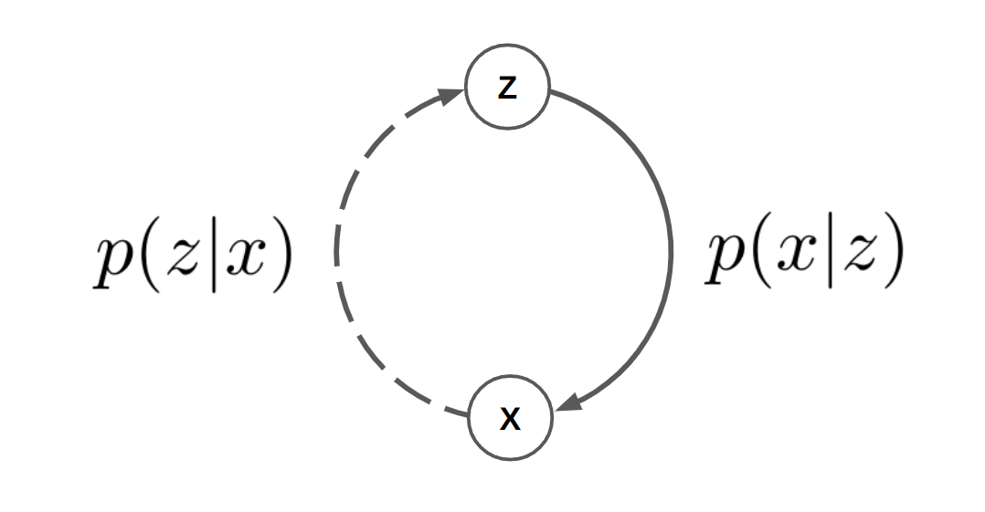
\[p(z|x) = \frac{p(x|z)p(z)}{p(x)}\]Graphically, the generative model $p(x | z)$ goes from the latent variables to the observation, while the inferred posterior $p(z | x)$ takes us from the observation to the latent variables:
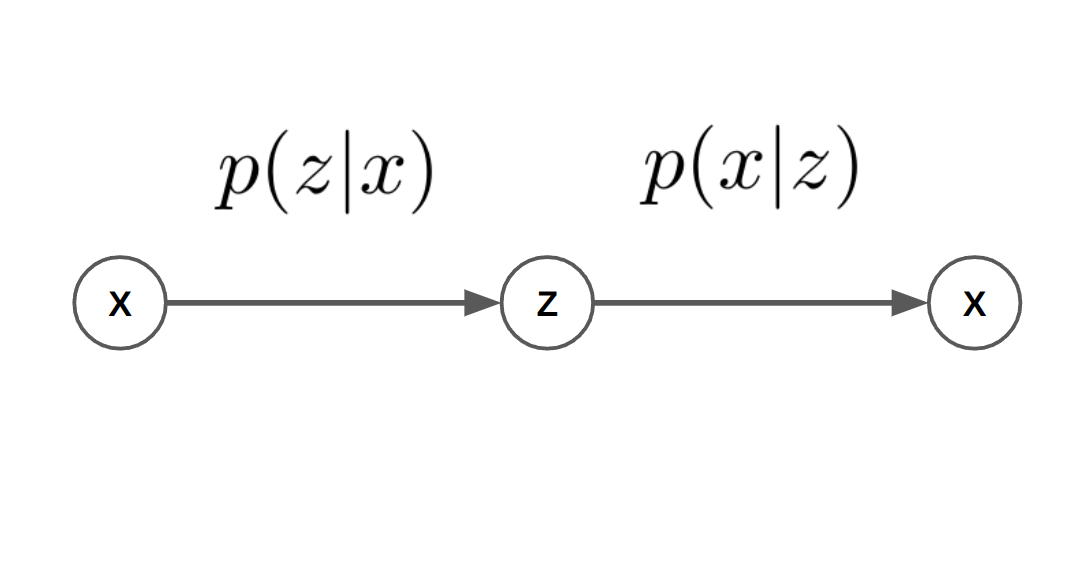
We can see the connection to autoencoders by “unrolling” this model. Given an observation, the “encoder” is now inference of the latent variables $z$, and “decoding” is conditioning on the latent variables:
An Approximation
Unfortunately, $p(z | x)$ tends to be hard to work with. The marginal probability $p(x)$ that appears in the denominator is typically unknown – or it may require exponential time to integrate over all the latent variables, i.e.,
\[p(x) = \int p(x|z)p(z) dz\]Variational Autoencoders take their name from Variational Inference, a powerful technique for approximating intractable probability distributions. The core idea of variational inference is to define a family of simpler, tractable distributions, and then use optimization to choose the best approximation within that family.
Instead of working with the (intractable) distribution $p(z | x)$, variational inference proposes a variational distribution $q( z | x)$. You can think of $q$ as a family of distributions with parameters $\phi$, and I’ll sometimes write $q( z | x; \phi)$ to make that explicit. For example, $q$ may be the family of Gaussian distributions, with $\phi$ being the mean and variance. The goal of variational inference is to choose $\phi$ so that $q( z | x; \phi)$ is as close to $p( z | x)$ as possible.
The “Closeness” of Distributions
In order to find a distribution that is “close” to $p(z | x)$, we need to define what we mean by close. The Kullback-Leibler (KL) Divergence is an information theoretic measure of how well one distribution approximates another. For continuous distributions, it’s usually written as
\[\begin{align} D_{KL}( P || Q) &= \int P(x) \log \frac{P(x)}{Q(x)} \, dx \\ &= \mathbb{E}_{x \sim P} \Big[ \log \frac{P(x)}{Q(x)} \Big] \end{align}\]where $P$ is the true distribution and $Q$ is the approximate. The intuition is clearer if we work with entropies instead of integrals or expectations:
\[D_{KL}( P || Q) = H(P,Q) - H(P)\]where
-
$H(P) = - \mathbb{E}_{x \sim P} [ \log P(x) ]$ is the entropy of $P$. It represents the uncertainty in $P$, and is the average number of bits needed to communicate a symbol drawn from the distribution.
-
$H(P,Q) = - \mathbb{E}_{x \sim P} [ \log Q(x) ]$ is the cross-entropy of $Q$ relative to $P$. It represents the average number of bits needed to communicate a symbol drawn from $P$ when it is encoded with respect to $Q$.
Together, the above equation shows that $D_{KL}(P || Q)$ is the average number of additional bits needed communicate a symbol drawn from $P$ when it is encoded with respect to $Q$. With this intuition, it makes sense that the KL divergence is always non-negative, and that it is zero only when $P = Q$. Note that $D_{KL}$ is not symmetric: $D_{KL}(P || Q) \ne D_{KL}(Q || P)$.
An Optimization
Putting the pieces together: Given observations $x$, we’d like to know the (intractable) posterior distribution $p(z | x; \theta)$. Instead, we have chosen a family of tractable distributions $Q$, and we want to find the distribution $q* \in Q$ that best approximates $P(Z | X)$. Let’s try doing this by minimizing the KL divergence,
\[q* = \arg \min_{q \in q(z | x; \phi)} D_{KL} \Big( p(z | x) || q(z | x; \phi) \Big)\]Unfortunately, $D_{KL}( p(z | x) || q(z | x; \phi))$ still requires us to take expectations with respect to the posterior $p(z | x)$, which we are assuming is intractable. Instead, we’ll minimize the Reverse KL divergence, $D_{KL}(Q || P)$,
\[q* = \arg \min_{q \in q(z | x; \phi)} D_{KL} \Big( q(z | x; \phi) || p(z | x) \Big)\]This won’t give us the same optima, but we will still get something that is “close” to $p(z|x)$ in a meaningful sense (see [1] for details). Let’s see what we can do with it. To reduce clutter, I’m going to write $q(z | x)$ as just $q$ for now,
\[\begin{align} D_{KL} \Big( q || p(z|x) \Big) &= H (q, p(z|x)) - H ( q) \\ &= H (q, p(x|z) ) + H(q, p(z) ) - H(q, p(x) ) - H( q) \\ &= H (q, p(x|z) ) + D_{KL} ( q || p(z)) - H(q , p(x) ) \\ &= H (q, p(x|z) ) + D_{KL} ( q || p(z)) + \log p(x) \geq 0 \end{align}\]The first step uses Bayes’ rule and substitutes $p(z|x) = p(x|z)p(z) / p(x)$ into the formula for cross-entropy. The second step regroups terms into $D_{KL} ( q(z|x) || p(z))$. The third step uses the fact that for the given x, $p(x)$ is constant. The inequality in the last line follows directly from the fact that $D_{KL}$ is non-negative.
Rearranging gives us a nice lower bound on the log likelihood:
\[\begin{align} \log p(x) &\geq -H (q(z|x), p(x|z) ) - D_{KL} ( q(z|x) || p(z)) \end{align}\]This is known as the Evidence Lower Bound, or ELBO. The cross-entropy term can be interpreted as a “reconstruction loss”: given $x$, it is the expected number of additional bits needed to communicate that x, when when we sample $z \sim q(z | x)$ and encode $x$ w.r.t $p(x|z)$. The KL-divergence term can be viewed as a regularizer that encourages the approximate posterior $q(z|x)$ to be close to the prior $p(z)$.
The model $(\theta, \phi)$ is learned by maximizing this lower bound.
A Variational Autoencoder
In this section, we will use neural network layers to learn the probabilistic encoder and decoder. The encoder will learn the approximate posterior $q(z | x; \phi)$, and the decoder will learn the generative model $p(x | z; \theta)$. We will choose the form of the variational distribution $q(z | x; \phi)$, …. , and train the VAE on the MNIST dataset using PyTorch.
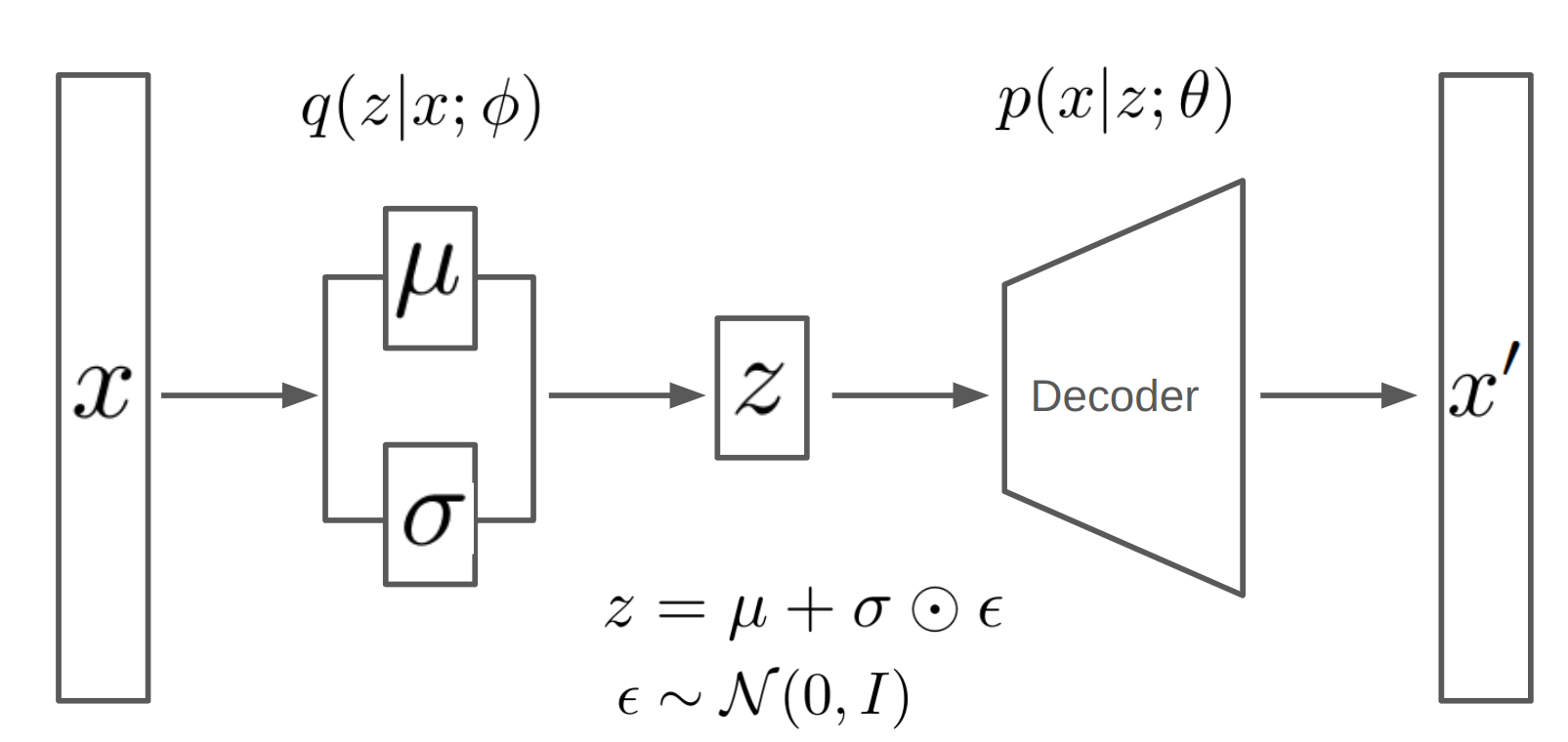
Following [2], we assume Gaussian distributions:
- $p(z) = \mathcal{N}(z; 0, I)$
- $ p(x | z; \theta) = \mathcal{N}(x; \mu_x(z), \Sigma_x(z))$
- $ q(z | x; \phi) = \mathcal{N}(z; \mu_z(x), \sigma_z(x)^2 I) $
We will use the encoder neural network to learn the functions $\mu_z(x)$ and $\sigma_z^2$, and the decoder neural network will learn the function $\mu_x(z)$ ($\Sigma_x(z)$ is assumed to be i.i.d pixel noise).
Building on the convolutional autoencoder from the previous post, the ConvolutionalVAE uses almost the same convolutional layers in the encoder and decoder. The main change is that the encoder outputs both $\mu_z$ and $\sigma_z$, each of length code_size, as opposed to a single latent vector of length `code_size’.
class ConvolutionalVAE(nn.Module):
    def __init__(self, code_size: int) -> None:
        super(ConvolutionalVAE, self).__init__()
        self.code_size = code_size

        # Encoder outputs mu and log(sigma^2) of the latent code.
        # log(sigma^2) is used instead of sigma^2 to avoid possible
        # numerical issues with small values.
        self.encoder = nn.Sequential(
            # [B, 1, 28, 28] -> [B, 16, 14, 14]
            nn.Conv2d(1, 16, 3, stride=2, padding=1),
            nn.ReLU(True),

            # [B, 16, 14, 14] -> [B, 32, 7, 7]
            nn.Conv2d(16, 32, 3, stride=2, padding=1),
            nn.ReLU(True),

            # [B, 32, 7, 7] -> [B, code_size * 2, 1, 1]
            nn.Conv2d(32, code_size * 2, 7),
        )

        # Decoder outputs the mean of the output data.
        self.decoder = nn.Sequential(
            # [B, code_size, 1, 1] -> [B, 32, 7, 7]
            nn.ConvTranspose2d(code_size, 32, 7),
            nn.ReLU(True),

            # [B, 32, 7, 7] -> [B, 16, 14, 14]
            nn.ConvTranspose2d(32, 16, 3, stride=2, padding=1, output_padding=1),
            nn.ReLU(True),

            # [B, 16, 14, 14] -> [B, 1, 28, 28]
            nn.ConvTranspose2d(16, 1, 3, stride=2, padding=1, output_padding=1),
            nn.Sigmoid(),  # To bring the output between [0, 1]
        )

    def encode(self, x: Tensor) -> Tuple[Tensor, Tensor]:
        """
        Encode the input data x into the mean and log of the variance of the latent code.

        :param x: Input tensor of shape (batch_size, input_size)
        :return: mu_z, log_variance_z
        """
        mu_z, log_variance_z = self.encoder(x).chunk(2, dim=1)
        return mu_z, log_variance_z

    def sample_z(self, mu_z: Tensor, log_variance_z: Tensor) -> Tensor:
        """
        Sample the latent code z from the mean and log of the variance of the latent code.

        :param mu_z: Mean of the latent code.
        :param log_variance_z: Log of the variance of the latent code.
        :return: Sampled latent code z.
        """
        # sigma = exp(log(sigma)), and log(sigma) = log(sigma^2) / 2
        sigma = torch.exp(0.5 * log_variance_z)
        epsilon = torch.randn_like(sigma)
        # This is the "reparametrization trick"
        z = mu_z + epsilon * sigma
        return z

    def decode(self, z: Tensor) -> Tensor:
        """
        Decode the latent code z into the mean of the output data.

        :param z: Latent code tensor of shape (batch_size, code_size)
        :return: mu_x
        """
        mu_x: Tensor = self.decoder(z)
        return mu_x

    def forward(self, x: Tensor) -> Tuple[Tensor, Tensor, Tensor]:
        """
        Forward pass of the VAE model.

        :param x: Input tensor of shape (batch_size, input_size)
        :return: mu_x, mu_z, log_variance_z
        """

        mu_z, log_variance_z = self.encode(x)
        z = self.sample_z(mu_z, log_variance_z)
        mu_x = self.decode(z)
        return mu_x, mu_z, log_variance_z

    def generate(self, num_samples: int, device) -> Tensor:
        """
        Generate new samples from the VAE model.

        :param num_samples: Number of samples to generate.
        :param device: Device to use.
        :return: Generated samples.
        """

        # Sample noise from a standard normal distribution.
        z = torch.randn(num_samples, self.code_size).to(device)
        # Convert z to a tensor of shape (num_samples, code_size, 1, 1)
        z = z.view(-1, self.code_size, 1, 1)
        samples: Tensor = self.decoder(z)
        return samples
Loss Function
Returning to our objective function,
\[\begin{align} \log p(x) &\geq -H (q(z|x), p(x|z) ) - D_{KL} ( q(z|x) || p(z)) \end{align}\]In some cases, the KL divergence term can be integrated analytically. That’s the case here, and is actually the case whenever $q(z|x)$ and $p(z)$ are from the exponential family.
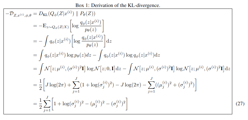
In code,
def vae_loss(
    x: torch.Tensor, x_prime: torch.Tensor, mu: torch.Tensor, log_variance: torch.Tensor
) -> torch.Tensor:
    """
    Loss function for the Variational Autoencoder (VAE), assuming a Gaussian prior and approximate posterior.

    :param x: Input data.
    :param x_prime: Reconstructed data.
    :param mu: Mean of the latent code.
    :param log_variance: Log of the variance of the latent code.
    :return: Sum of binary cross-entropy loss and KL divergence loss.
    """
    # Sum of binary cross-entropy loss over all elements of the batch.
    reconstruction_loss: Tensor = F.binary_cross_entropy(x_prime, x, reduction='sum')

    # KL Divergence
    # Appendix B of Kingma and Welling gives an analytical solution for the KL divergence when
    # 1. The prior is the standard normal distribution, i.e. p_{\theta}(z) = N(z; 0, I)
    # 2. The approximate posterior distribution q_{\phi}(z|x) is Gaussian with mean mu and diagonal covariance matrix sigma^2

    # Sum of KL divergence over all elements of the batch.
    # 0.5 * sum(1 + log(sigma^2) - mu^2 - sigma^2)
    kl_divergence: Tensor = -0.5 * torch.sum(1 + log_variance - mu.pow(2) - log_variance.exp())

    return reconstruction_loss + kl_divergence
Training and Evaluation
Following the paper, the latent code size is 20. The rest of the training configuration is similar to that in previous posts:
device = torch.device("cuda" if torch.cuda.is_available() else "cpu")

    # === Configuration ===

    # Path to the directory where downloaded data is stored.
    data_path = "./data"

    # Training batch size.
    batch_size = 100

    # Number of passes over the training data.
    num_epochs = 200

    # Learning rate for the optimizer.
    learning_rate = 1e-3

    latent_code_size = 20

    # === Data ===
    transform = transforms.Compose([transforms.ToTensor()])  # Converts pixel values in the range [0, 255] to [0, 1].
    train_loader, test_loader = mnist(data_path, batch_size, transform)

    vae = ConvolutionalVAE(latent_code_size).to(device)
    summary(vae, input_size=(batch_size, 1, 28, 28))

    # === Training ===

    vae.train()
    vae.to(device)
    optimizer = optim.Adam(vae.parameters(), lr=learning_rate)

    for epoch in range(num_epochs):
        print(f"Epoch [{epoch + 1}/{num_epochs}]")
        epoch_loss = 0.0
        for images, _labels in train_loader:
            images = images.to(device)

            # Forward pass
            outputs, mu, sigma = vae(images)
            batch_loss = vae_loss(images, outputs, mu, sigma)
            epoch_loss += batch_loss.item()

            # Backward pass and parameter updates
            optimizer.zero_grad()
            batch_loss.backward()
            optimizer.step()

        avg_train_loss = epoch_loss / float(len(train_loader.dataset))
        print(f"  Average Training Loss: {avg_train_loss:.8f}")
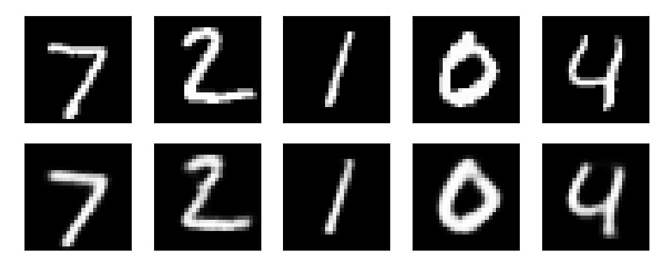
The reconstructed images are unsurprising:
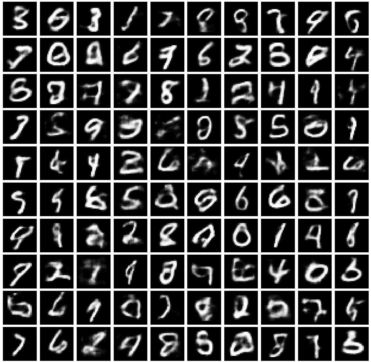
More interesting, though, are images generated by the network. These are created by sampling a latent vector $z \sim \mathcal{N}(0,1)$ and feeding it through the decoder. There’s some junk in there, but a number of them are convincing digits.
References and Further Reading
- An Introduction to Variational Inference
- Autoencoding Variational Bayes
- Chapter 13: Approximate Inference, Deep Learning
- PyTorch VAE example