Deep Learning: Convolutional Neural Nets
The previous post trained an autoencoder for the MNIST images of handwritten digits. While that worked, it was a very generic solution in the sense that it ignored the spatial structure of an image and just treated an image as a vector of numbers. This time, we’ll build a convolutional autoencoder that uses convolutional layers instead of fully-connected layers. Convolutional layers offer several advantages over fully-connected layers, and are particularly good for image processing.
Convolutional layers use a set of learnable filters (or kernels) that are applied across the entire input. Each filter is spatially smaller than the input but extends through the full depth of the input (e.g., all color channels in an image). This design allows convolutional layers to share weights across different spatial locations, drastically reducing the number of parameters compared to fully-connected layers. Reducing the number of parameters helps prevent overfitting and makes the model more efficient. Sharing weights across spatial locations also makes convolutional layers inherently translation invariant, meaning that they can recognize patterns regardless of where they appear in the input. This is because the same filter is applied across the entire input, making the network less sensitive to the location of the features.
Let’s take a look at some code:
class ConvAutoencoder(nn.Module):
    def __init__(self) -> None:
        super(ConvAutoencoder, self).__init__()

        # Encoder: Conv2d layers
        self.encoder = nn.Sequential(
            # [B, 1, 28, 28] -> [B, 16, 14, 14]
            nn.Conv2d(1, 16, 3, stride=2, padding=1),
            nn.ReLU(True),

            # [B, 16, 14, 14] -> [B, 32, 7, 7]
            nn.Conv2d(16, 32, 3, stride=2, padding=1),
            nn.ReLU(True),

            # [B, 32, 7, 7] -> [B, 12, 1, 1]
            nn.Conv2d(32, 12, 7),
        )

        # Decoder: ConvTranspose2d layers
        self.decoder = nn.Sequential(
            # [B, 12, 1, 1] -> [B, 32, 7, 7]
            nn.ConvTranspose2d(12, 32, 7),
            nn.ReLU(True),

            # [B, 32, 7, 7] -> [B, 16, 14, 14]
            nn.ConvTranspose2d(32, 16, 3, stride=2, padding=1, output_padding=1),
            nn.ReLU(True),

            # [B, 16, 14, 14] -> [B, 1, 28, 28]
            nn.ConvTranspose2d(16, 1, 3, stride=2, padding=1, output_padding=1),
            # Map the output to [0, 1]
            nn.Sigmoid(),
        )

    def forward(self, x: Tensor) -> Tuple[Tensor, Tensor]:
        """
        Forward pass of the autoencoder model.
        Args:
            x: Input tensor of shape (batch_size, 1, 28, 28)

        Returns: Output, latent code

        """
        z = self.encoder(x)
        x_prime: Tensor = self.decoder(z)
        return x_prime, z
Like the previous autoencoder, this model is also composed of an encoder that maps the input into a lower-dimensional representation – the latent space or code – and a decoder that reconstructs the input data from this lower-dimensional code.
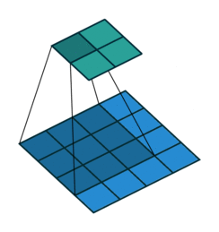
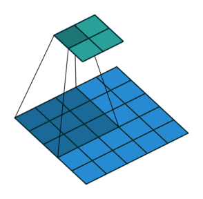
Instead of fully-connected layers, the encoder now uses Conv2d layers. The convolutions are strided: they progressively reduce the spatial dimensions of the input image while using the depth (number of channels) of each layer to learn features. Strided convolutions are an alternative to pairing a convolutional layer with a downsampling layer like max pooling (see Striving for Simplicity: the All Convolutional Net).
The decoder is largely the “reverse” of the encoder. It uses ConvTranspose2d layers to upsample the latent code back into a 28 x 28 pixel image.
Training and Evaluation
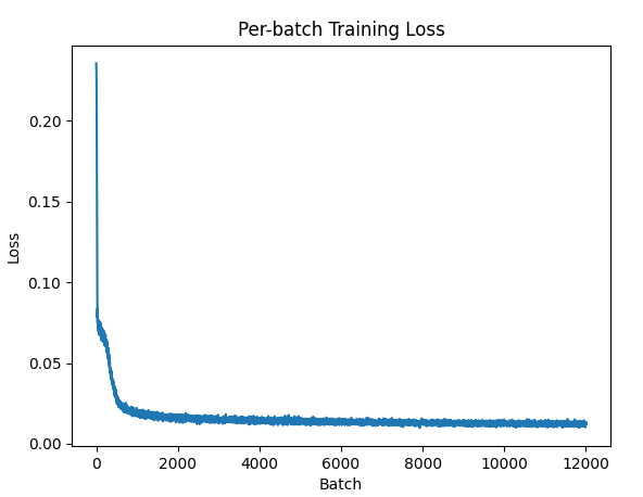
The training loss looks quite nice:
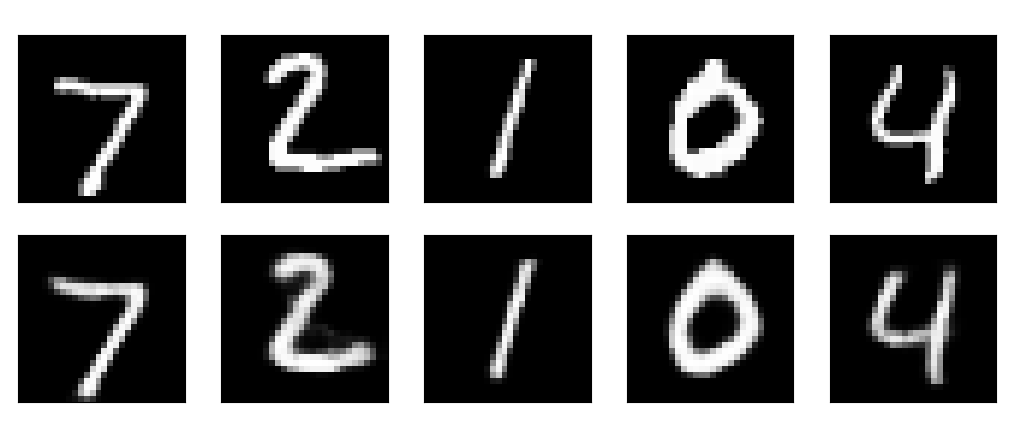
Finally, let’s see how it looks. The top row of figures are the inputs, and the bottom row are output reconstructions. For a bottleneck size of 12, this is about a 65:1 compression.
References and Further Reading
- Striving for Simplicity: the All Convolutional Net
- A Guide to Convolution Arithmetic for Deep Learning