Deep Learning: Autoencoders
Today, I want to kick off a series of posts about Deep Learning. As the first installment, this post delves into the fundamentals of autoencoders, their applications, and gives a worked example of training an autoencoder with PyTorch.
Learning a low-dimensional representation
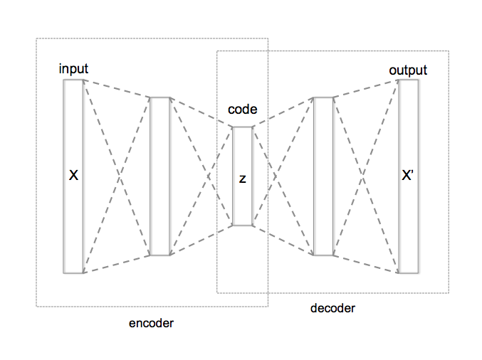
An autoencoder is a type of neural network used to learn an efficient coding of the input data in an unsupervised manner. The primary goal of an autoencoder is to transform inputs into outputs with minimal loss, which involves encoding the input into a compressed, latent representation and then reconstructing the output from this representation. If you think about image compression algorithms, a good compression function compresses a large image to a smaller size, but does it in a way that lets us later recover a good approximation of the original image. An autoencoder simultaneously learns the compression and decompression functions — or, more traditionally, the encoder and the decoder:
- Encoder: Maps the input data to a lower-dimensional representation (the latent space or “code”).
- Decoder: Reconstructs the input data from this lower-dimensional representation.
In addition to dimensionality reduction, the autoencoder’s ability to learn a meaningful representation of data is useful for denoising; learning features as pre-training for a supervised learning task; or, in the case of variational autoencoders, generating new data that is similar to the training examples.
Training an AutoEncoder with PyTorch
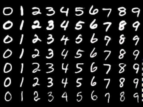
Let’s start with a small example of training an autoencoder on the venerable MNIST handwritten digits dataset, consisting of 28 x 28 pixel, grayscale images of handwitten digits. The dataset contains 60,000 training images and 10,000 testing images. “The digits have been size-normalized and centered in a fixed-size image. It is a good database for people who want to try learning techniques and pattern recognition methods on real-world data while spending minimal efforts on preprocessing and formatting.” They look like this:
Network Architecture
The standard autoencoder NN has a simple structure designed for compression: it’s basically any network that “pinches down” in the middle to form a “bottleneck” between the encoder and the decoder.
For simplicity, I’ve chosen a “symmetric” autoencoder, parametrized by the number of layers and the width of each layer. All layers except the last use ReLU activations. ReLU is a good default choice: it is extremely simple and tends to propagate stable gradients during backpropagation. The final layer of the decoder uses a Tanh activation function in order to coerce the outputs back into grayscale pixel values.
class SymmetricAutoencoder(nn.Module):
    def __init__(self, layer_sizes: List[int]) -> None:
        """
        An Autoencoder with "mirrored" encoder and decoder architecture.

        The decoder is the mirror of the encoder. The first layer size must be
        the input size, and the last layer size must be the code size. layer_sizes
        must have at least 2 elements. This ensures that the input size and
        code size are specified.

        :param layer_sizes: List of layer sizes for the encoder.
        """

        super(SymmetricAutoencoder, self).__init__()
        # The input size and code size must be specified.
        if len(layer_sizes) < 2:
            raise ValueError("layer_sizes must have at least 2 elements.")

        # Encoder
        encoder_layers: List[nn.Module] = []
        input_size = layer_sizes[0]
        for i, output_size in enumerate(layer_sizes[1:]):
            encoder_layers.append(nn.Linear(input_size, output_size))
            encoder_layers.append(nn.ReLU())
            input_size = output_size
        self.encoder = nn.Sequential(*encoder_layers)

        # Decoder
        decoder_layers: List[nn.Module] = []
        reversed_layer_sizes = layer_sizes.copy()
        reversed_layer_sizes.reverse()
        input_size = reversed_layer_sizes[0]
        for i, output_size in enumerate(reversed_layer_sizes[1:]):
            decoder_layers.append(nn.Linear(input_size, output_size))
            if i < len(layer_sizes) - 2:  # Add ReLU for all but the last layer
                decoder_layers.append(nn.ReLU())
            input_size = output_size
        # Add tanh to the last layer to clamp the range of the output to [-1, 1].
        decoder_layers.append(nn.Tanh())
        self.decoder = nn.Sequential(*decoder_layers)

    def forward(self, x: Tensor) -> Tuple[Tensor, Tensor]:
        """
        Forward pass of the autoencoder model.

        :param x: input tensor of shape (batch_size, input_size)
        :return: Output, latent code
        """
        code = self.encoder(x)
        recovered = self.decoder(code)
        return recovered, code
Bottleneck: PCA and Cumulative Explained Variance
One of the main challenges in training an autoencoder is ensuring that it does not simply learn the identity function, where the output is identical to the input without meaningful compression. The simplest way to avoid this is to create a “bottleneck” layer between the encoder and the decoder that is smaller than the size of the input. This ensures that some meaningful compression takes place.
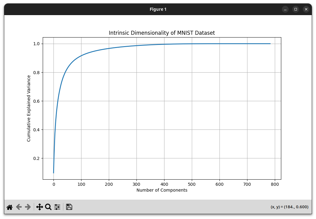
So, how should we choose the size of the bottleneck layer? Unlike most parameters, we can’t just do grid search to find the “best” size: increasing the bottleneck size only makes it easier for the network to reproduce its inputs. Instead, we could ask, how small can the bottleneck be, while still giving a required level of accuracy? An effective method to guide this decision is Principal Component Analysis (PCA), a linear dimensionality reduction technique that can help identify the intrinsic dimensionality of the data. PCA transforms data into a set of orthogonal components, ordered by the amount of variance they “explain” or “capture” from the data. Taking the first k principal components amounts to projecting the data onto the k-dimensional subspace that preserves the most variance. Plotting the fraction of the cumulative variance explained by the first k principal components gives a nice way of seeing how many dimensions we need to represent our dataset reasonably well. This is sometimes called the intrinsic dimension of the data.
For the MNIST dataset, k=154 components are enough to explain 95% of the variance.
   # Perform PCA and calculate the cumulative explained variance.
    pca = PCA()
    pca.fit(data)
    explained_variance_ratio = np.cumsum(pca.explained_variance_ratio_)

    # The number of components needed to explain 95% of the variance
    n_components_95 = np.where(explained_variance_ratio >= 0.95)[0][0] + 1
    print(f'Number of components to explain 95% variance: {n_components_95}')
How many layers?
The Universal Approximator Theorem tells us that even a single hidden layer can be quite powerful: “One major advantage of nontrivial depth is that the universal approximator theorem guarantees that a feed-forward neural network with at least one hidden layer can represent an approximation of any function (within a broad class) to an arbitrary degree of accuracy, provided that it has enough hidden units.” With the input size fixed and the bottleneck size chosen via PCA, that leaves us freedom to choose the number and widths of additional hidden layers. I did a little grid search over those values, using K-fold cross validation compare models. Among the configurations I offered, the best model had a single additional layer, of width 2500, between the input and the bottleneck.
def k_fold_cross_validation(
        k: int,
        dataset: Dataset,
        model_factory: Callable[[], SymmetricAutoencoder],
        device: torch.device,
        criterion: nn.Module,
        batch_size: int,
        learning_rate: float,
        num_epochs: int) -> List[float]:
    """
    Perform k-fold cross-validation.
    :param k: Number of folds.
    :param dataset: Dataset to split into k folds.
    :param model_factory: Factory function for the model.
    :param device: Device to run the model on.
    :param criterion: Loss function.
    :param batch_size: Training batch size.
    :param learning_rate: Learning rate for the optimizer.
    :param num_epochs: Number of training epochs.
    :return: Average validation loss on each fold.
    """

    kfold = KFold(n_splits=k, shuffle=True)

    # Validation loss of each folding.
    validation_losses = []

    for fold, (train_indices, val_indices) in enumerate(kfold.split(dataset)):
        print(f'Fold {fold}')

        train_subset = Subset(dataset, train_indices)
        validation_subset = Subset(dataset, val_indices)

        train_loader = DataLoader(train_subset, batch_size=batch_size, shuffle=True, num_workers=4)
        validation_loader = DataLoader(validation_subset, batch_size=batch_size, shuffle=False, num_workers=4)

        model = model_factory().to(device)
        optimizer = optim.Adam(model.parameters(), lr=learning_rate)

        train_autoencoder(model, device, train_loader, optimizer, num_epochs)
        loss = evaluate_autoencoder(model, device, validation_loader, criterion)
        validation_losses.append(loss)

    return validation_losses
Training with Stochastic Gradient Descent
PyTorch makes the actual training of neural networks extremely easy. The snippet below performs stochastic gradient descent using the Adam optimizer. Adam is short for “Adaptive Moment Estimation”, and the key idea of the algorithm is that it adjusts the learning rate of each parameter based on estimates of the first and second moments of the gradients. This has the effect of “averaging out” noisy gradient estimates (e.g., due to small batch sizes), and of reducing the step size when there is high uncertainty about a parameter’s gradient. This is all pretty boilerplate, but if it is new to you, the key point is that backpropagation and differentiable objective functions make it “easy” to train neural networks. This post is probably my favorite on the topic.
    criterion: nn.MSELoss = nn.MSELoss()
    layers = [image_size, 150]
    model: SymmetricAutoencoder = SymmetricAutoencoder(image_size).cuda()
    summary(model, input_size=(batch_size, image_size))
    optimizer = optim.Adam(model.parameters(), lr=learning_rate)
    per_batch_loss: List[float] = train_autoencoder(model, device, train_loader, optimizer, num_epochs)
def train_autoencoder(
        model: nn.Module,
        device: torch.device,
        train_loader: DataLoader,
        optimizer: torch.optim.Optimizer,
        num_epochs: int
) -> List[float]:
    """
    Train the autoencoder model.
    :param model: Initial model. This model will be modified during training.
    :param device: Device to run the model on.
    :param train_loader: training data loader. Data must be a tuple (inputs, labels).
    :param optimizer: Optimizer for training.
    :param num_epochs: Number of epochs for training.
    :return: Per-batch training loss.
    """

    # Per-batch training loss. This includes batches from all epochs.
    per_batch_loss: List[float] = []

    # === Training ===
    model.train()
    for epoch in range(num_epochs):

        # Average batch loss in this epoch.
        epoch_avg_batch_loss = 0.0

        start_time = time.time()
        # Iterate over training batches.
        for inputs, _labels in train_loader:
            inputs = inputs.to(device)

            # Forward pass
            outputs, _code = model(inputs)
            loss = nn.MSELoss()
            loss = loss(outputs, inputs)
            epoch_avg_batch_loss += loss.item()
            per_batch_loss.append(loss.item())

            # Backward pass and parameter updates
            optimizer.zero_grad()
            loss.backward()
            optimizer.step()

        elapsed_time = time.time() - start_time
        num_batches = len(train_loader)
        epoch_avg_batch_loss /= num_batches
        print(
            f'Epoch [{epoch + 1}/{num_epochs}], Averge Loss per Batch: {epoch_avg_batch_loss:.4f}, Time: {elapsed_time:.2f} seconds')

    return per_batch_loss
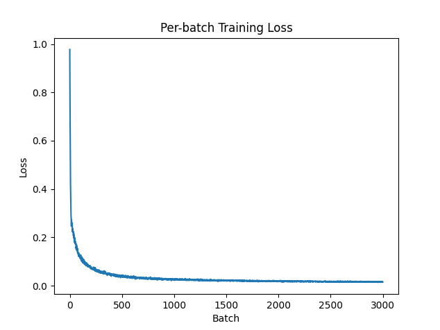
The training loss looks quite nice:
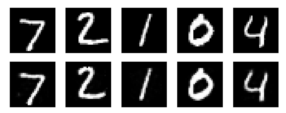
Evaluation
Finally, let’s see how it looks. The top row of figures are the inputs, and the bottom row are output reconstructions. For a bottleneck size of 150, this is about a 5.2:1 data compression.
References and Further Reading
- Deep Learning, Goodfellow et. al., 2016, Chapter 14: Autoencoders
- The MNIST Database
- Rectified Linear Units Improve Restricted Boltzmann Machines
- Adam: A Method for Stochastic Optimization
- Calculus on Computational Graphs: Backpropagation