Deep Learning: Transformers
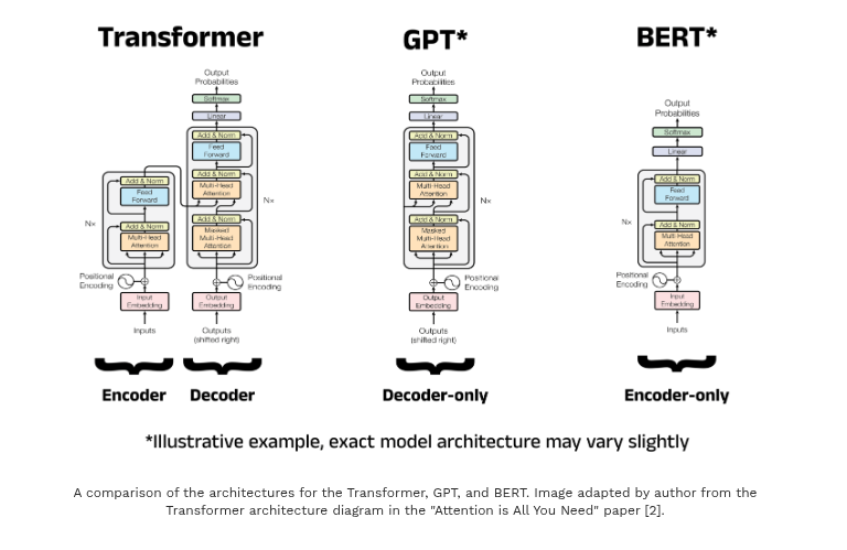
This post is a detailed look at the original Transformer. We’ll be working through the intuition, architecture, and a PyTorch implementation. By the end, you should be able to train and run your own transformer, and feel comfortable with each component in this diagram:
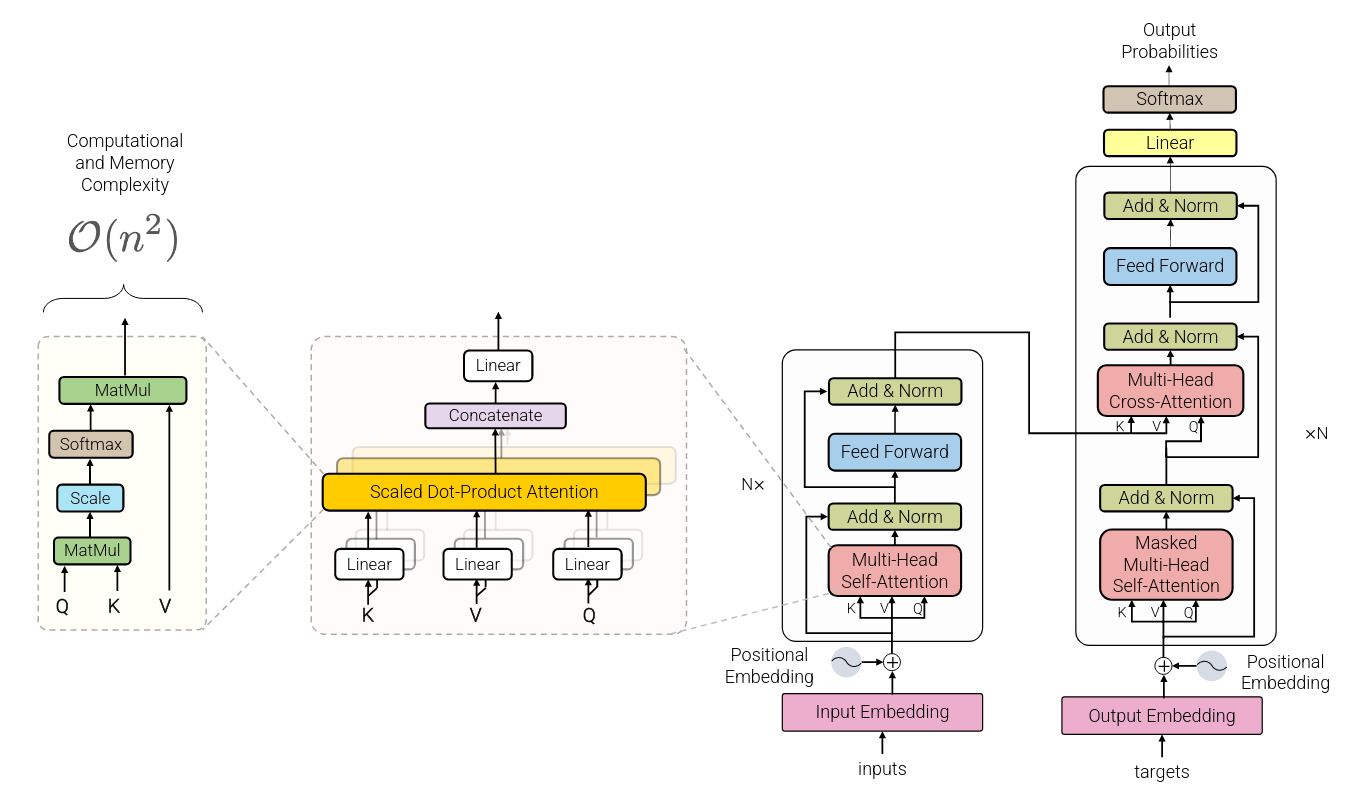
The Transformer
In less than a decade, transformers have become the dominant architecture in modern machine learning, spanning text embedding models for search and retrieval, large language models for generation, and models for images, audio, and protein structure. Introduced by Vaswani et al. in the 2017 paper Attention Is All You Need, the transformer architecture replaced recurrence and convolution with a single mechanism: attention. Earlier sequence models like RNNs and LSTMs compressed all prior information into a fixed-length hidden state, forcing the network to distill an entire sequence into a single vector. In contrast, the transformer computes a representation of each position in the sequence by letting it directly “attend to” every other position, drawing in context from the parts of the input most relevant to it.
This section steps through the definition and implementation of each part of the diagram:
- Attention
- Scaled dot product attention
- Multi-Head Attention
- QKV projections
- Positional embeddings
- Masking
- Layer norm / dropout
- The feed-forward network
- Embeddings and the output head
- Stacking blocks into a full encoder-decoder model
- Training it, and generating from it
Before getting started, let’s define some symbols for the dimensions involved, and import some things we’ll use in the code snippets:
# Dimensions

# B    Batch size
# T    Sequence length
# T_q  When computing cross-attention, sequence length corresponding to queries
# T_k  When computing cross-attention, sequence length corresponding to keys and values
# D    Dimension of keys and queries, often written d_k
# d_v  Dimension of values. This post assumes d_v = D
# H    Attention head dimension
from typing import Optional, Tuple
import math

import torch
import torch.nn as nn
import torch.nn.functional as F
If Attention is All You Need, What Don’t You Need? Recurrence.
“We propose a new simple network architecture, the Transformer, based solely on attention mechanisms, dispensing with recurrence and convolutions entirely”
Before transformers, most sequence-to-sequence models relied on recurrent neural networks (RNNs) and their more sophisticated variants like Long Short-Term Memory (LSTM) and Gated Recurrent Units (GRUs). These architectures process sequences one element at a time, updating a hidden state as each new element arrives. This design gives RNNs a natural sense of order but also serious limitations: long-range dependencies are difficult to capture, gradients tend to vanish over many time steps, and the inherently sequential nature of recurrence makes training slow and difficult to parallelize.
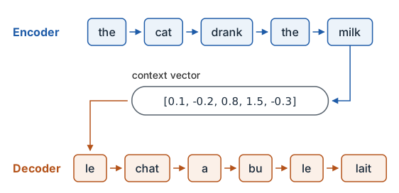
A specific example: The sequence-to-sequence model introduced by Sutskever et al. (2014) extended RNNs into an encoder-decoder framework, where the encoder compressed the entire input sequence into a single fixed-length context vector, and the decoder generated the output sequence from it. This worked well for short sentences, but as the sequences grow longer, that single vector becomes a bottleneck, forcing the network to represent all relevant information in a narrow space. Transformers break from this paradigm. Instead of a fixed-length context vector, transformers process all elements of the sequence simultaneously and model the relationships between each pair of them using a mechanism called attention.
Attention
Attention allows a model to dynamically focus on the most relevant parts of its input when making each decision, weighting information based on how strongly it relates to the current context.
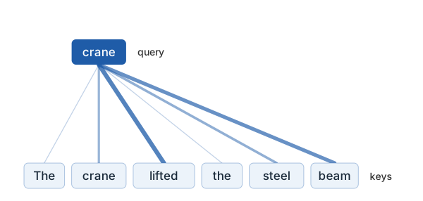
Attention was first introduced in the context of neural machine translation as a way to overcome the limitations of fixed-length context vectors used in early encoder–decoder models. In Neural Machine Translation by Jointly Learning to Align and Translate (Bahdanau et al., 2014), the authors proposed allowing the decoder to “softly search” through all positions of the input sequence at each step of translation—deciding dynamically which parts of the input were most relevant to the word being generated. This replaced the rigid, one-size-fits-all summary of the source sentence with a flexible mechanism that could focus on different words at different times. Subsequent refinements, such as Luong et al. (2015)’s Effective Approaches to Attention-Based Neural Machine Translation, further formalized this idea, showing that attention consistently improved translation quality, especially for long or complex sentences.
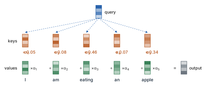
At its core, attention is a method for computing a weighted average over a set of elements, where the weights are determined dynamically based on the relationship between an input query and each element’s representation. Each element in the sequence is represented by a key and a value—the key describing what the element is about, and the value carrying the actual content we might want to retrieve. The query is another vector in the same feature space, representing what we’re looking for. The attention mechanism measures how relevant each key is to the query, typically using a similarity function such as a dot product. Elements whose keys are most similar to the query receive higher weights, meaning the model “attends” to them more strongly.
Scaled Dot Product Attention
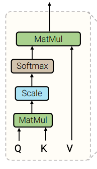
Formally, this process can be viewed as mapping a query and a set of key–value pairs to an output vector. The relevance scores between the query and each key are computed via dot products, scaled for numerical stability, and passed through a softmax function to form a probability distribution over the elements. The final output is then a weighted sum of the values — effectively the expected value of the sequence given the query. This is known as scaled dot-product attention.
For a single query vector $q$, a set of keys $K = [k_1, k_2, \dots, k_T]$, and corresponding values $V = [v_1, v_2, \dots, v_T]$, scaled dot-product attention is defined as
\[\text{Attention}(q, K, V) = \text{softmax}\!\left(\frac{qK^T}{\sqrt{d_k}}\right)V\]where
- $q \in \mathbb{R}^{d_k}$ is the query vector,
- $K \in \mathbb{R}^{T \times d_k}$ are the keys,
- $V \in \mathbb{R}^{T \times d_v}$ are the values,
- $d_k$ is the dimensionality of the keys and queries, and
- $d_v$ is the dimensionality of the values.
The scaling term $\sqrt{d_k}$ in the denominator serves to normalize the magnitude of the dot products between queries and keys. Without it, when the dimensionality $d_k$ is large, the dot products tend to grow in magnitude, pushing the softmax function into regions where it becomes extremely peaked. As a result, gradients vanish and learning slows. We can see this by looking at the gradients of the softmax function w.r.t. its inputs. Recall that the softmax of a vector $z$ is given by
\[s_i = \text{softmax}(\mathbf{z})_i = \frac{e^{z_i}}{ \sum_{j = 1}^N e^{z_j}}\]Because every output depends on every input, the derivative is a full Jacobian rather than a single number. Differentiating gives
\[\frac{\partial s_i}{\partial z_j} = s_i \left( \delta_{ij} - s_j \right)\]where $\delta_{ij}$ is $1$ when $i = j$ and $0$ otherwise. Thomas Kurbiel works the derivation through step by step in Derivative of the Softmax Function and the Categorical Cross-Entropy Loss. Writing the entries out for $N = 4$ makes the structure visible:
\[J_{\text{softmax}} = \begin{pmatrix} s_1(1 - s_1) & -s_1 s_2 & -s_1 s_3 & -s_1 s_4 \\ -s_2 s_1 & s_2(1 - s_2) & -s_2 s_3 & -s_2 s_4 \\ -s_3 s_1 & -s_3 s_2 & s_3(1 - s_3) & -s_3 s_4 \\ -s_4 s_1 & -s_4 s_2 & -s_4 s_3 & s_4(1 - s_4) \end{pmatrix}\]The diagonal entries take the form $s_i(1 - s_i)$ and the off-diagonal entries $-s_i s_j$, but either way every entry carries a factor of some $s$.
When softmax saturates, a single $s_i$ value approaches 1, and the others approach $0$, and the gradients all vanish. Dividing by $\sqrt{d_k}$ counteracts this effect by keeping the variance of the dot products roughly constant, ensuring that attention weights remain well-scaled and that the model can learn effectively across different embedding dimensions.
In code:
def scaled_dot_product_attention(
    q: torch.Tensor,   # (d_k,)
    K: torch.Tensor,   # (T, d_k)
    V: torch.Tensor,   # (T, d_v)
) -> Tuple[torch.Tensor, torch.Tensor]:
    """
    Scaled dot-product attention for a single query.

    Returns:
        Tuple[torch.Tensor, torch.Tensor]:
            - context (torch.Tensor): The attention output, a weighted sum
              of values with shape (d_v,).
            - weights (torch.Tensor): The attention weights (probabilities)
              over the T keys with shape (T,).
    """
    T, d_k = K.size(0), K.size(1)
    # Scores over T keys: (T,)
    scores = torch.matmul(q, K.t()) / math.sqrt(d_k)

    # Attention weights over T positions: (T,)
    # Subtracting scores.max() improves numerical stability by preventing overflow in exp()
    weights = F.softmax(scores - scores.max(), dim=0)

    # Weighted sum of values: (d_v,)
    context = torch.matmul(weights.unsqueeze(0), V).squeeze(0)

    return context, weights
Self-Attention
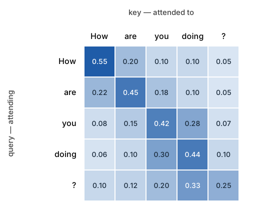
So far, our attention mechanism takes a sequence of elements (i.e., keys and values) and a query, and returns a single value. We can extend this mechanism by associating a query with each element, so we can compute how much each element “attends” to every other element:
\[\text{Attention}(Q, K, V) = \text{softmax}\!\left(\frac{QK^T}{\sqrt{d_k}}\right)V\]The matrix multiplication $QK^T$ performs the dot product for every possible pair of queries and keys, resulting in a matrix of shape $T \times T$.
That $T \times T$ matrix is the cost of giving up recurrence, and it is the $\mathcal{O}(n^2)$ annotation in the diagram at the top of this post. An RNN processes a sequence in time linear in its length but cannot parallelize across it; attention parallelizes completely but computes and stores a score for every pair of positions. Doubling the sequence length quadruples both the work and the memory, which is why context length is the expensive dimension to scale and why a long line of later work — sparse, linear, and flash attention among it — is concerned with computing this matrix without materializing all of it.
In the special case where the queries, keys, and values all come from the same sequence, we call this self-attention. Self-attention allows every element in a sequence to attend to every other element, including itself. This means that each element’s representation is updated based on a weighted combination of all elements in the sequence, where the weights reflect their relevance to that element.
Let’s update the implementation of scaled_dot_product_attention to compute attention for multiple queries, and allow for an optional dimension for batches:
def scaled_dot_product_attention(
    Q: torch.Tensor,  # (T, d_k) or (B, T, d_k)
    K: torch.Tensor,  # (T, d_k) or (B, T, d_k)
    V: torch.Tensor,  # (T, d_v) or (B, T, d_v)
) -> Tuple[torch.Tensor, torch.Tensor]:
    """
    Scaled dot-product attention (multiple queries, optional batching)

    Returns:
        context: (T, d_v) or (B, T, d_v)
        weights: (T, T) or (B, T, T)
    """
    # Validate ranks
    if Q.dim() not in (2, 3) or K.dim() != Q.dim() or V.dim() != Q.dim():
        raise ValueError("Q, K, V must all be rank-2 (T,D) or rank-3 (B,T,D) tensors of the same rank.")

    # Validate inner dims
    if Q.size(-1) != K.size(-1):
        raise ValueError(f"Query/key dims must match: {Q.size(-1)} != {K.size(-1)}")
    if K.size(-2) != V.size(-2):
        raise ValueError(f"Time dims of K and V must match: {K.size(-2)} != {V.size(-2)}")

    # Normalize to 3D: (B, T, D) where B=1 for unbatched
    def _to_3d(x):
        return x.unsqueeze(0) if x.dim() == 2 else x

    Q3, K3, V3 = _to_3d(Q), _to_3d(K), _to_3d(V)
    d_k = Q3.size(-1)

    # Scores: (B, T, T)
    scores = torch.matmul(Q3, K3.transpose(-2, -1)) / math.sqrt(d_k)

    # Attention weights
    weights = F.softmax(scores, dim=-1) # Softmax over keys

    # Context: (B, T, d_v)
    context = torch.matmul(weights, V3)

    # Restore to original rank
    if Q.dim() == 2:
        context = context.squeeze(0)   # (T, d_v)
        weights = weights.squeeze(0)   # (T, T)

    return context, weights
Multi-Head Attention
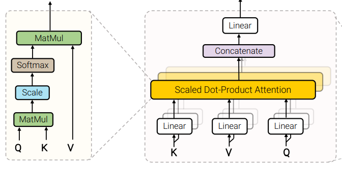
Scaled dot-product attention gives us a powerful primitive: given a query, we compute a weighted average over a set of values based on their relevance. However, a single attention operation forces the model to express all relationships in one shared representation space. In practice, different types of relationships—such as syntactic structure, semantic similarity, or positional alignment—can interfere with one another when compressed into a single set of attention weights. Multi-head attention addresses this limitation by running several attention operations in parallel, each with its own learned projections of queries, keys, and values.
Intuitively, each attention “head” can be thought of as looking at the sequence from a different perspective. One head might learn to attend to nearby words, another to long-range dependencies, and another to specific structural patterns like subject–verb agreement. Because each head operates on a lower-dimensional subspace, the model can represent diverse relationships simultaneously without forcing them into a single attention map. The outputs of these heads are then combined, allowing the model to integrate multiple views of the same sequence into a richer representation.
Casually, multi-head attention is a fancy name for running several (smaller) attention instances in parallel.
Formally, multi-head attention applies $h$ independent scaled dot-product attention operations. Given input matrices $Q \in \mathbb{R}^{T \times D}$, $K \in \mathbb{R}^{T \times D}$, and $V \in \mathbb{R}^{T \times D}$, we first project them using learned linear transformations:
\[Q_i = Q W_i^Q \in \mathbb{R}^{T \times H}, \quad K_i = K W_i^K \in \mathbb{R}^{T \times H}, \quad V_i = V W_i^V \in \mathbb{R}^{T \times H}\]Here, $H$ is the dimension of each head, often chosen as $H = D / h$ so that the total computational cost remains similar to that of single-head attention with dimension $D$.
Each head computes scaled dot-product attention independently:
\[\text{head}_i = \text{Attention}(Q W_i^Q,\; K W_i^K,\; V W_i^V)\]The resulting head outputs are concatenated and linearly transformed once more:
\[\text{MultiHead}(Q, K, V) = \text{Concat}(\text{head}_1, \dots, \text{head}_h)\, W^O\]where $W^O \in \mathbb{R}^{(h \cdot H) \times D}$.
Back to the code. Let’s extend scaled_dot_product_attention to accept a tensor with leading dimensions for batching and heads:
Note the two sequence lengths in the signature. Self-attention draws queries, keys, and values from the same sequence, so T_q == T_k; cross-attention draws the queries from a different sequence, so the two can differ. Writing them separately keeps the decoder’s cross-attention working without a second implementation.
def scaled_dot_product_attention(
    Q: torch.Tensor,                     # (B, H, T_q, d_k)
    K: torch.Tensor,                     # (B, H, T_k, d_k)
    V: torch.Tensor,                     # (B, H, T_k, d_v)
    mask: Optional[torch.Tensor] = None, # broadcastable to (B, H, T_q, T_k)
    dropout_p: float = 0.0,
    training: bool = True,
) -> Tuple[torch.Tensor, torch.Tensor]:
    """
    Compute scaled dot-product attention

    Args:
        Q: Queries of shape (B, H, T_q, d_k)
        K: Keys    of shape (B, H, T_k, d_k)
        V: Values  of shape (B, H, T_k, d_v)
        mask: Optional attention mask, broadcastable to (B, H, T_q, T_k).
              - If boolean: True means "keep/allow", False means "mask out".
              - If floating: additive mask (e.g., 0 for keep, -inf for mask),
                added to the attention scores before softmax.
        dropout_p: Dropout probability applied to attention weights.
        training:  If true, dropout is applied

    Returns:
        context: Weighted sum of values, shape (B, H, T_q, d_v)
        attn:    Attention weights over keys, shape (B, H, T_q, T_k)
    """
    d_k = Q.size(-1)

    # Scores: (B, H, T_q, T_k)
    scores = torch.matmul(Q, K.transpose(-2, -1)) / math.sqrt(d_k)

    # Masking
    if mask is not None:
        if mask.dtype == torch.bool:
            scores = scores.masked_fill(~mask, float("-inf"))
        else:
            scores = scores + mask

    # Numerical stability: subtract per-row max so exp() doesn't overflow (softmax is shift-invariant).
    scores = scores - scores.max(dim=-1, keepdim=True).values

    # Attention weights: (B, H, T_q, T_k)
    attn = F.softmax(scores, dim=-1)

    # Optional dropout on attention weights
    if dropout_p and dropout_p > 0.0:
        attn = F.dropout(attn, p=dropout_p, training=training)

    # Context: (B, H, T_q, d_v)
    context = torch.matmul(attn, V)

    return context, attn
class MultiHeadAttention(nn.Module):
    """
    Multi-head attention module.

    Shapes:
      - Input:  x_q: (B, T_q, d_model)
                x_k: (B, T_k, d_model)  (defaults to x_q if not provided)
                x_v: (B, T_k, d_model)  (defaults to x_k if not provided)
      - Mask:   broadcastable to (B, H, T_q, T_k)
      - Output: y:   (B, T_q, d_model)
                attn:(B, H, T_q, T_k)

    Notes:
      - This is the "standard" Transformer MHA: per-head d_k = d_v = d_model / num_heads.
      - For tutorial clarity, d_model must be divisible by num_heads.
    """

    def __init__(self, d_model: int, num_heads: int, dropout_p: float = 0.0, bias: bool = True):
        """
          Args:
            d_model: Total embedding of the input and output tensors.
            num_heads: Number of attention heads. d_model must be divisible by num_heads.
            dropout_p: Dropout probability applied to the attention weights.
            bias: If true, include additive bias terms in the linear projections.
        """
        super().__init__()
        if d_model % num_heads != 0:
            raise ValueError(f"d_model must be divisible by num_heads; got d_model={d_model}, num_heads={num_heads}")

        self.d_model = d_model
        self.num_heads = num_heads
        self.d_head = d_model // num_heads
        self.dropout_p = float(dropout_p)

        # Q/K/V projections are implemented as single "packed" linear layers.
        # Conceptually, each head h has its own projection W_h^Q, W_h^K, W_h^V
        # with shape (d_model, d_head). In practice we concatenate the H per-head
        # matrices along the output dimension to form one matrix:
        #
        #   W^Q = [W_1^Q | W_2^Q | ... | W_H^Q] ∈ R^{d_model × (H·d_head)} = R^{d_model × d_model}
        #
        # so applying nn.Linear(d_model, d_model) produces an output of shape
        # (B, T, H·d_head), which we then reshape into (B, H, T, d_head) to recover
        # the per-head queries/keys/values.
        self.W_q = nn.Linear(d_model, d_model, bias=bias)
        self.W_k = nn.Linear(d_model, d_model, bias=bias)
        self.W_v = nn.Linear(d_model, d_model, bias=bias)

        # Output projection that mixes information across heads.
        # After attention, per-head outputs are concatenated back into
        # a (B, T, d_model) tensor; this linear layer projects that
        # concatenated representation back into the model space.
        self.W_o = nn.Linear(d_model, d_model, bias=bias)

        self._reset_parameters()

    def _reset_parameters(self) -> None:
        """
        Xavier (Glorot) uniform initialization for the four projections.

        nn.Linear defaults to Kaiming-uniform, which is scaled for ReLU-style
        activations. The attention projections have no activation, so Xavier's
        fan_in/fan_out scaling is the better match: it keeps the variance of
        the activations roughly constant across the projection, which in turn
        keeps the pre-softmax scores in a range where the softmax gradient has
        not yet saturated.
        """
        for proj in (self.W_q, self.W_k, self.W_v, self.W_o):
            nn.init.xavier_uniform_(proj.weight)
            if proj.bias is not None:
                nn.init.zeros_(proj.bias)

    def _split_heads(self, x: torch.Tensor) -> torch.Tensor:
        """
        Split the model dimension into multiple attention heads.

        This reshapes and permutes a tensor from (B, T, d_model) into
        (B, H, T, d_head), where d_head = d_model / H.
        """
        B, T, _ = x.shape
        x = x.view(B, T, self.num_heads, self.d_head)
        return x.transpose(1, 2)  # (B, H, T, d_head)

    def _combine_heads(self, x: torch.Tensor) -> torch.Tensor:
        """
        Combine multiple attention heads back into the model dimension.

        This permutes and reshapes a tensor from (B, H, T, d_head) into
        (B, T, d_model) by concatenating the head dimensions.
        """
        B, H, T, d_head = x.shape
        x = x.transpose(1, 2).contiguous()  # (B, T, H, d_head)
        return x.view(B, T, H * d_head)

    def forward(
        self,
        x_q: torch.Tensor,                        # (B, T_q, d_model)
        x_k: Optional[torch.Tensor] = None,       # (B, T_k, d_model)
        x_v: Optional[torch.Tensor] = None,       # (B, T_k, d_model)
        mask: Optional[torch.Tensor] = None,      # broadcastable to (B, H, T_q, T_k)
        return_attn: bool = False,
    ) -> torch.Tensor | Tuple[torch.Tensor, torch.Tensor]:
        """
        Args:
            x_q: Query input, shape (B, T_q, d_model)
            x_k: Key input,   shape (B, T_k, d_model). Defaults to x_q (self-attention).
            x_v: Value input, shape (B, T_k, d_model). Defaults to x_k.
            mask: Optional mask broadcastable to (B, H, T_q, T_k).
            return_attn: If True, also return attention weights (B, H, T_q, T_k).

        Returns:
            y: (B, T_q, d_model)
            attn (optional): (B, H, T_q, T_k)
        """
        if x_k is None:
            x_k = x_q
        if x_v is None:
            x_v = x_k

        # Project to model dim, then split into heads.
        Q = self._split_heads(self.W_q(x_q))  # (B, H, T_q, d_head)
        K = self._split_heads(self.W_k(x_k))  # (B, H, T_k, d_head)
        V = self._split_heads(self.W_v(x_v))  # (B, H, T_k, d_head)

        # Attention per head.
        context, attn = scaled_dot_product_attention(
            Q, K, V, mask=mask, dropout_p=self.dropout_p, training=self.training
        )  # context: (B, H, T_q, d_head)

        # Recombine heads and project out.
        y = self.W_o(self._combine_heads(context))  # (B, T_q, d_model)

        if return_attn:
            return y, attn
        return y
Keys, Values, Queries?
- Keys, Values, Queries aren’t given, they’re computed via projection matrices
- Where did these matrices come from? They’re learned jointly with the rest of the model
- Meta-lesson: the architecture can assume that functions exist, and then learn them into existence
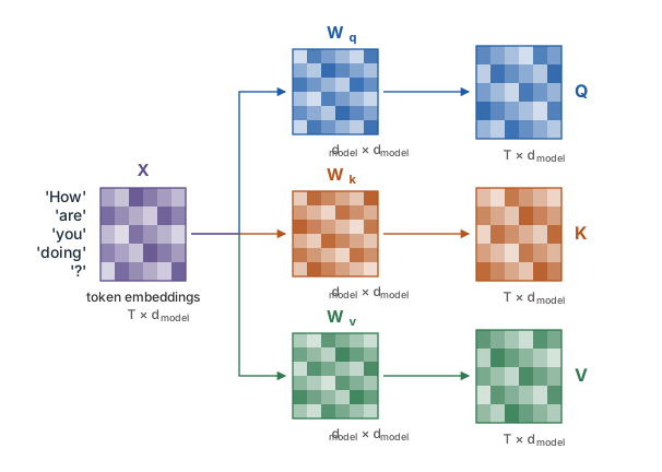
So far we have talked about queries, keys, and values as though they were given — each element arriving with a key describing what it is about and a value carrying its content. Look at what forward actually receives: a single tensor x_q of shape (B, T, d_model), and in the self-attention case that one tensor supplies the keys and values too. Keys, values, and queries aren’t given. They’re computed, via the projection matrices self.W_q, self.W_k, and self.W_v.
The three projections map the same input into three different subspaces, so a single element representation can act as a query when asking what it needs from the sequence, a key when advertising what it offers, and a value when delivering its content. The separation also makes the relationship directional: with one projection producing both queries and keys, $QK^T$ would be symmetric, and “the verb attends to its subject” would carry exactly the same weight as “the subject attends to its verb.”
Where did these matrices come from? They’re learned jointly with the rest of the model. W_q, W_k, and W_v are nn.Linear layers like any other. The training objective says nothing about what makes a good key or a good query; the only signal is the loss at the output, and the projections arrive at whatever notion of relevance reduces it.
Meta-lesson: Attention assumes that a useful notion of relevance exists, then learns it into existence.
Positional Embeddings
Attention computes a weighted average over a set of elements, and nothing in that computation refers to where an element sits in the sequence. The scores come from $QK^T$, which compares content against content, and the output sums over all positions. Permute the input and the output permutes the same way, with every value unchanged. Writing $P$ for a permutation matrix,
\[\text{Attention}(PQ, PK, PV) = P \cdot \text{Attention}(Q, K, V)\]because the $P^T P$ introduced by $(PQ)(PK)^T$ cancels. The feed-forward sublayer applies to each position independently, so it preserves the property as well. As far as the architecture is concerned, “the cat sat on the mat” and “the mat sat on the cat” are the same bag of words.
The fix in Attention Is All You Need is to put position into the representation itself, by adding a positional encoding to each input embedding before the first layer:
\[x_t = \sqrt{d_{\text{model}}} \cdot \text{Embedding}(w_t) + \text{PE}_t\]The encoding is built from sinusoids of geometrically increasing wavelength. For position $t$ and embedding dimension $i$:
\[\text{PE}_{(t,\, 2i)} = \sin\!\left(\frac{t}{10000^{2i/d_{\text{model}}}}\right), \qquad \text{PE}_{(t,\, 2i+1)} = \cos\!\left(\frac{t}{10000^{2i/d_{\text{model}}}}\right)\]Each pair of dimensions holds one sinusoid, and the wavelengths run from $2\pi$ in the lowest pair up to $10000 \cdot 2\pi$ in the highest. Low dimensions oscillate quickly and distinguish neighboring positions; high dimensions oscillate slowly and distinguish regions of a long sequence.
Why sinusoids, rather than feeding the raw index $t$ as a feature? The values stay in $[-1, 1]$ regardless of sequence length, so they do not swamp the embedding they are added to. The encoding has no parameters and is defined for every $t$, so a model can be run on sequences longer than any it saw in training. And for any fixed offset $k$, the angle-addition identities make $\text{PE}_{t+k}$ a linear function of $\text{PE}_t$ — a rotation by an angle that depends only on $k$, not on $t$. The paper hypothesized that this is what lets the model learn to attend by relative position.
In code:
class PositionalEncoding(nn.Module):
    """
    Fixed sinusoidal positional encoding.

    The table is precomputed and registered as a buffer, so it moves with
    .to(device) and is saved in the state dict without being a parameter.
    """

    def __init__(self, d_model: int, max_len: int = 5000, dropout_p: float = 0.0):
        """
        Args:
            d_model: Embedding dimension. Must be even, so that each sinusoid
                     occupies one (sin, cos) pair of dimensions.
            max_len: Largest sequence length the table is built for.
            dropout_p: Dropout applied to the sum of embedding and encoding.
        """
        super().__init__()
        if d_model % 2 != 0:
            raise ValueError(f"d_model must be even; got d_model={d_model}")

        self.dropout = nn.Dropout(p=dropout_p)

        # Positions t = 0, 1, ..., max_len - 1
        t = torch.arange(max_len).unsqueeze(1)          # (max_len, 1)

        # 10000^(-2i/d_model), computed in log space for numerical stability.
        div = torch.exp(
            torch.arange(0, d_model, 2) * (-math.log(10000.0) / d_model)
        )                                               # (d_model/2,)

        pe = torch.zeros(max_len, d_model)
        pe[:, 0::2] = torch.sin(t * div)                # even dimensions
        pe[:, 1::2] = torch.cos(t * div)                # odd dimensions

        self.register_buffer("pe", pe.unsqueeze(0))     # (1, max_len, d_model)

    def forward(self, x: torch.Tensor) -> torch.Tensor:
        """
        Args:
            x: (B, T, d_model), embeddings already scaled by sqrt(d_model).

        Returns:
            (B, T, d_model)
        """
        T = x.size(1)
        if T > self.pe.size(1):
            raise ValueError(f"sequence length {T} exceeds max_len {self.pe.size(1)}")
        return self.dropout(x + self.pe[:, :T])
The encoding is added to the embeddings rather than concatenated, which costs no extra dimensions and lets every layer above see position information mixed into the same $d_{\text{model}}$ channels.
Learned absolute embeddings replace the table with an nn.Embedding(max_len, d_model) trained like any other parameter — simpler to state, and used by BERT and GPT-2, but defined only up to max_len. Rotary position embeddings (RoPE) take a different route: instead of adding anything to the input, they rotate the query and key vectors inside each attention operation by an angle proportional to position, so the dot product between a query and a key depends directly on their separation. RoPE is the common choice in current large language models.
Masking
Attention lets every query see every key, which is sometimes more than we want.
A decoder generates one element at a time, and the representation it builds for position $t$ must depend only on positions $1 \dots t$. If position $t$ could attend to position $t+1$ during training, the model would learn to read the answer off the input, and training would not match generation, where later positions do not exist yet.
Padding is the other case. Sequences in a batch rarely have the same length, so shorter ones are padded to a common $T$. Those padding slots hold no content, and a query that attends to them is averaging in noise.
Both are handled the same way: before the softmax, set the scores of disallowed query-key pairs to $-\infty$. The softmax maps $-\infty$ to a weight of exactly zero, so those keys contribute nothing to the weighted average and receive no gradient. This is what the mask branch in scaled_dot_product_attention does, with a boolean mask marking which pairs are allowed.
The mask only has to be broadcastable to (B, H, T_q, T_k), which keeps both kinds cheap. A causal mask does not depend on the batch or the head, so it is built once at (1, 1, T, T). A padding mask depends on the batch but applies to every head and every query, so it is (B, 1, 1, T_k):
def causal_mask(T: int, device: Optional[torch.device] = None) -> torch.Tensor:
    """
    Allow each query to attend to itself and to earlier keys only.

    Returns a (1, 1, T, T) boolean mask, broadcastable over batch and heads.
    """
    allowed = torch.ones(T, T, dtype=torch.bool, device=device).tril()
    return allowed.view(1, 1, T, T)


def padding_mask(lengths: torch.Tensor, T_k: int) -> torch.Tensor:
    """
    Block key positions that are padding rather than content.

    Args:
        lengths: (B,) number of real elements in each sequence of the batch.
        T_k: Padded key-sequence length.

    Returns a (B, 1, 1, T_k) boolean mask, broadcastable over heads and queries.
    """
    idx = torch.arange(T_k, device=lengths.device)         # (T_k,)
    allowed = idx.unsqueeze(0) < lengths.unsqueeze(1)      # (B, T_k)
    return allowed.view(lengths.size(0), 1, 1, T_k)
Both follow the convention the attention code already expects: True means “attend to this”, False means “mask it out”. Because they are booleans, combining them is just a logical and, and broadcasting produces the (B, 1, T, T) mask a decoder needs:
mask = causal_mask(T, device=x.device) & padding_mask(lengths, T)
The three masks in the encoder-decoder blocks below follow from this. The encoder masks only padding, since an encoder is free to look at the whole source sequence in both directions. The decoder’s self_mask is causal, combined with padding if the target is batched. The decoder’s cross_mask is padding over the source keys and is not causal — there is no reason to hide part of the input from the decoder, only part of the output.
Caveat: If a query row is masked out entirely, every score in that row is $-\infty$, and the softmax over them is $0/0$. The result is NaN, which then spreads through the rest of the network. This happens when a padding mask is applied along the query axis as well as the key axis, so that padded queries have nothing left to attend to. The usual fix is to leave the query axis unmasked, as padding_mask above does, and drop the padded positions later when computing the loss.
Layer Normalization and Dropout
Layer normalization and dropout appear throughout the blocks below without being part of the attention computation. Neither changes what a block can represent; both are there to make deep stacks of blocks trainable.
Layer Normalization
Layer normalization standardizes each position’s feature vector on its own. For the representation $x \in \mathbb{R}^{d_{\text{model}}}$ at a single position,
\[\mu = \frac{1}{d_{\text{model}}}\sum_{i=1}^{d_{\text{model}}} x_i, \qquad \sigma^2 = \frac{1}{d_{\text{model}}}\sum_{i=1}^{d_{\text{model}}} (x_i - \mu)^2\] \[\text{LayerNorm}(x) = \gamma \odot \frac{x - \mu}{\sqrt{\sigma^2 + \epsilon}} + \beta\]where $\gamma$ and $\beta$ are learned vectors of length $d_{\text{model}}$, initialized to ones and zeros, and $\epsilon$ is a small constant guarding the division. Applied to a tensor of shape (B, T, d_model), nn.LayerNorm(d_model) reduces over the last axis only, so it performs $B \times T$ independent normalizations — one per position of each sequence.
Compare batch normalization, which standardizes each feature across the examples in a batch. That makes an example’s output depend on whatever else it was batched with. For sequences that is awkward: a batch holds sequences of different lengths, so the statistics are computed over a mixture of real content and padding, and they shift with batch size. Batch norm also has to keep running averages to behave sensibly at inference, where there may be no batch to compute statistics over. Layer norm has none of these problems. It looks at one position at a time, so it behaves identically for a batch of 256 and a batch of 1, and identically in training and evaluation.
Where to put the normalization is a separate choice: before each sublayer, or after the residual addition. We come back to it after the encoder block below.
Dropout
Dropout zeroes each element of a tensor independently with probability $p$ during training, and scales the survivors by $1/(1-p)$ so that the expected value is unchanged. At evaluation time it is the identity. The transformer applies it in three places, all of which appear in the code in this post:
- On the sum of the embeddings and the positional encoding, at the bottom of each stack. This is the
dropout_pargument toPositionalEncodingabove. - On each sublayer’s output, before the residual addition —
x = x + self.dropout(attn_out)in the blocks below. The residual path itself is never dropped, so there is always a clean route for the gradient. - On the attention weights, inside
scaled_dot_product_attention. This severs individual query-key connections at random, so a query cannot come to depend on any single key. It also leaves the attention rows no longer summing to one.
The first two are what Vaswani et al. describe; dropout on the attention weights comes from the reference implementations and is now standard. The base model in the paper used $p = 0.1$ in all of them.
Because dropout behaves differently in training and evaluation, it matters that the blocks hold nn.Dropout modules rather than calling F.dropout directly. model.eval() switches a module off automatically, while the functional form needs its training flag supplied by the caller — which is why scaled_dot_product_attention takes one and MultiHeadAttention passes training=self.training down to it.
The Feed-Forward Network
Attention moves information between positions, but it does little to that information along the way. Once the weights are fixed, the output at each position is a weighted average of value vectors, which is a linear operation. The feed-forward sublayer is the other half of every block, and it supplies the nonlinearity:
self.ffn = nn.Sequential(
    nn.Linear(d_model, d_ff, bias=bias),
    nn.GELU() if activation.lower() == "gelu" else nn.ReLU(),
    nn.Linear(d_ff, d_model, bias=bias),
)
Two linear layers with an activation between them, projecting up to a wider dimension $d_{ff}$ and back down. The paper used $d_{ff} = 4 \cdot d_{\text{model}}$ — 2048 against a model dimension of 512 — and the ratio has stuck.
It is applied position-wise: the same two matrices run over every position independently, with no mixing across the sequence. That is what makes the permutation argument from the positional embeddings section go through, and it means all cross-position communication in a transformer happens in exactly one place, the attention sublayer.
Most of the parameters live here too. Each block spends $2 \cdot d_{\text{model}} \cdot d_{ff}$ parameters on the feed-forward network against $4 \cdot d_{\text{model}}^2$ on the four attention projections, so at the usual $d_{ff} = 4 \cdot d_{\text{model}}$ the feed-forward network is twice the size of the attention it accompanies.
Encoder-Decoder
class EncoderBlock(nn.Module):
    """
    A standard Transformer encoder block (pre-norm), composed of:

      1) Multi-head self-attention + residual
      2) Position-wise feed-forward network + residual

    This implementation uses "pre-norm" LayerNorm:
      x -> LN -> sublayer -> dropout -> residual add

    Shapes:
      x:    (B, T, d_model)
      mask: optional, broadcastable to (B, H, T, T) for self-attention

    Returns:
      y:    (B, T, d_model)
      attn: (B, H, T, T) if return_attn=True
    """

    def __init__(
        self,
        d_model: int,
        num_heads: int,
        d_ff: int,
        dropout_p: float = 0.0,
        activation: str = "gelu",
        bias: bool = True,
    ):
        """
        Initialize an encoder block.

        Args:
            d_model: Model/embedding dimension.
            num_heads: Number of attention heads.
            d_ff: Hidden dimension of the feed-forward network (FFN).
            dropout_p: Dropout probability applied after attention/FFN outputs.
            activation: Activation function in the FFN ("gelu" or "relu").
            bias: Whether to include bias terms in linear layers.
        """
        super().__init__()
        self.dropout_p = float(dropout_p)

        self.self_attn = MultiHeadAttention(d_model=d_model, num_heads=num_heads, dropout_p=dropout_p, bias=bias)

        self.norm1 = nn.LayerNorm(d_model)
        self.norm2 = nn.LayerNorm(d_model)

        self.ffn = nn.Sequential(
            nn.Linear(d_model, d_ff, bias=bias),
            nn.GELU() if activation.lower() == "gelu" else nn.ReLU(),
            nn.Linear(d_ff, d_model, bias=bias),
        )

        self.dropout = nn.Dropout(p=dropout_p)

    def forward(
        self,
        x: torch.Tensor,                    # (B, T, d_model)
        mask: Optional[torch.Tensor] = None, # broadcastable to (B, H, T, T)
        return_attn: bool = False,
    ) -> torch.Tensor | Tuple[torch.Tensor, torch.Tensor]:
        """
        Args:
            x: Input sequence embeddings, shape (B, T, d_model).
            mask: Optional attention mask broadcastable to (B, H, T, T).
            return_attn: If True, also return attention weights.

        Returns:
            y: Updated embeddings, shape (B, T, d_model).
            attn (optional): Attention weights, shape (B, H, T, T).
        """
        # ---- Self-attention sublayer (pre-norm) ----
        x_norm = self.norm1(x)
        if return_attn:
            attn_out, attn = self.self_attn(x_q=x_norm, mask=mask, return_attn=True)
        else:
            attn_out = self.self_attn(x_q=x_norm, mask=mask, return_attn=False)

        x = x + self.dropout(attn_out)

        # ---- Feed-forward sublayer (pre-norm) ----
        x_norm = self.norm2(x)
        ffn_out = self.ffn(x_norm)
        x = x + self.dropout(ffn_out)

        return (x, attn) if return_attn else x
The original Transformer paper, Attention Is All You Need, used the post-norm formulation, where LayerNorm is applied after each residual addition. This worked well for the relatively shallow models studied at the time (e.g., 6 encoder layers), but later work found that post-norm Transformers become increasingly difficult to train as depth grows, often requiring careful learning-rate warmup and tuning to remain stable. As a result, most modern implementations adopt the pre-norm variant, which applies LayerNorm before each sublayer. Pre-norm preserves an exact identity path through the residual connections, greatly improving gradient flow and making deep Transformers significantly more stable and easier to optimize, which is why it is now the default choice in practice.
from __future__ import annotations

from typing import Optional, Tuple
import torch
import torch.nn as nn


class DecoderBlock(nn.Module):
    """
    A standard Transformer decoder block (pre-norm), composed of:

      1) Masked multi-head self-attention + residual
      2) Cross-attention over encoder outputs + residual
      3) Position-wise feed-forward network + residual

    This implementation uses "pre-norm" LayerNorm:
      x -> LN -> sublayer -> dropout -> residual add

    Shapes:
      x:        (B, T, d_model)          decoder hidden states
      enc_out:  (B, S, d_model)          encoder outputs (source length S)
      self_mask:  optional, broadcastable to (B, H, T, T)   (typically causal and/or padding)
      cross_mask: optional, broadcastable to (B, H, T, S)   (typically padding over source keys)

    Returns:
      y:        (B, T, d_model)
      attn_self:  (B, H, T, T) if return_attn=True
      attn_cross: (B, H, T, S) if return_attn=True
    """

    def __init__(
        self,
        d_model: int,
        num_heads: int,
        d_ff: int,
        dropout_p: float = 0.0,
        activation: str = "gelu",
        bias: bool = True,
    ):
        """
        Initialize a decoder block.

        Args:
            d_model: Model/embedding dimension.
            num_heads: Number of attention heads.
            d_ff: Hidden dimension of the feed-forward network (FFN).
            dropout_p: Dropout probability applied after attention/FFN outputs.
            activation: Activation function in the FFN ("gelu" or "relu").
            bias: Whether to include bias terms in linear layers.
        """
        super().__init__()
        self.dropout_p = float(dropout_p)

        self.self_attn = MultiHeadAttention(d_model=d_model, num_heads=num_heads, dropout_p=dropout_p, bias=bias)
        self.cross_attn = MultiHeadAttention(d_model=d_model, num_heads=num_heads, dropout_p=dropout_p, bias=bias)

        self.norm1 = nn.LayerNorm(d_model)  # before self-attn
        self.norm2 = nn.LayerNorm(d_model)  # before cross-attn
        self.norm3 = nn.LayerNorm(d_model)  # before FFN

        self.ffn = nn.Sequential(
            nn.Linear(d_model, d_ff, bias=bias),
            nn.GELU() if activation.lower() == "gelu" else nn.ReLU(),
            nn.Linear(d_ff, d_model, bias=bias),
        )

        self.dropout = nn.Dropout(p=dropout_p)

    def forward(
        self,
        x: torch.Tensor,                          # (B, T, d_model)
        enc_out: torch.Tensor,                    # (B, S, d_model)
        self_mask: Optional[torch.Tensor] = None, # broadcastable to (B, H, T, T)
        cross_mask: Optional[torch.Tensor] = None,# broadcastable to (B, H, T, S)
        return_attn: bool = False,
    ) -> torch.Tensor | Tuple[torch.Tensor, torch.Tensor, torch.Tensor]:
        """
        Args:
            x: Decoder input (hidden states), shape (B, T, d_model).
            enc_out: Encoder outputs to attend over, shape (B, S, d_model).
            self_mask: Optional mask for decoder self-attention, broadcastable to (B, H, T, T).
            cross_mask: Optional mask for cross-attention, broadcastable to (B, H, T, S).
            return_attn: If True, also return (self_attn_weights, cross_attn_weights).

        Returns:
            y: Updated decoder states, shape (B, T, d_model).
            attn_self (optional): (B, H, T, T)
            attn_cross (optional): (B, H, T, S)
        """
        # ---- Masked self-attention (pre-norm) ----
        x_norm = self.norm1(x)
        if return_attn:
            self_out, attn_self = self.self_attn(x_q=x_norm, mask=self_mask, return_attn=True)
        else:
            self_out = self.self_attn(x_q=x_norm, mask=self_mask, return_attn=False)
        x = x + self.dropout(self_out)

        # ---- Cross-attention (pre-norm): queries from decoder, keys/values from encoder ----
        x_norm = self.norm2(x)
        if return_attn:
            cross_out, attn_cross = self.cross_attn(x_q=x_norm, x_k=enc_out, mask=cross_mask, return_attn=True)
        else:
            cross_out = self.cross_attn(x_q=x_norm, x_k=enc_out, mask=cross_mask, return_attn=False)
        x = x + self.dropout(cross_out)

        # ---- Feed-forward (pre-norm) ----
        x_norm = self.norm3(x)
        ffn_out = self.ffn(x_norm)
        x = x + self.dropout(ffn_out)

        if return_attn:
            return x, attn_self, attn_cross
        return x
Embeddings and the Output Head
Everything so far operates on vectors of width d_model. Real input is discrete — token ids — and real output is a distribution over a vocabulary. Converting between the two is the job of the pink boxes at the bottom of the diagram and the Linear/Softmax at the top.
Before the vocabulary holds any real words, it needs three reserved ids: one to pad short sequences, one to start the decoder off, and one for the model to emit when it is finished.
PAD, BOS, EOS = 0, 1, 2
An embedding table then maps each id to a learned vector:
self.src_embed = nn.Embedding(src_vocab_size, d_model, padding_idx=PAD)
self.tgt_embed = nn.Embedding(tgt_vocab_size, d_model, padding_idx=PAD)
padding_idx pins the row for PAD to zeros and keeps it from accumulating gradient, which pairs with the padding masks from earlier.
The paper then scales the embeddings by $\sqrt{d_{\text{model}}}$ before the positional encoding is added. That scaling only makes sense alongside a particular initialization, and the two are easy to separate by accident. The paper initializes the embedding matrix the way it initializes a linear layer, with entries of standard deviation around $d_{\text{model}}^{-1/2}$. Those are small enough that the $O(1)$ sinusoids would otherwise swamp them, and the $\sqrt{d_{\text{model}}}$ multiply restores the token signal to unit scale. PyTorch’s nn.Embedding does not initialize that way: its default is $\mathcal{N}(0, 1)$, so multiplying by $\sqrt{d_{\text{model}}}$ scales entries up by a factor of about 23 at $d_{\text{model}} = 512$, which is the opposite of the intent. Plenty of published implementations carry the multiply without the matching initialization. We set it explicitly so the two agree:
nn.init.normal_(self.src_embed.weight, mean=0.0, std=d_model ** -0.5)
nn.init.normal_(self.tgt_embed.weight, mean=0.0, std=d_model ** -0.5)
with torch.no_grad():                       # padding_idx is zeroed at init, not after
    self.src_embed.weight[PAD].zero_()
    self.tgt_embed.weight[PAD].zero_()
The difference is measurable. On the toy task at the end of this post, leaving the default initialization in place while keeping the $\sqrt{d_{\text{model}}}$ multiply costs roughly an order of magnitude in final loss, 0.0985 against 0.0059, and drops exact-match accuracy from 256/256 to 244/256.
At the top of the model, one linear layer projects back to vocabulary size:
self.out_proj = nn.Linear(d_model, tgt_vocab_size)
The diagram draws a softmax after it, but the module does not apply one. F.cross_entropy during training and argmax during decoding both work directly on the logits — the first is more numerically stable that way, and the second does not care, since softmax is monotonic.
Stacking the Blocks
The N× in the diagram is a stack of identical blocks, each feeding the next:
class Encoder(nn.Module):
    """A stack of N encoder blocks."""

    def __init__(self, num_layers: int, d_model: int, num_heads: int, d_ff: int,
                 dropout_p: float = 0.1, activation: str = "relu"):
        super().__init__()
        self.layers = nn.ModuleList([
            EncoderBlock(d_model=d_model, num_heads=num_heads, d_ff=d_ff,
                         dropout_p=dropout_p, activation=activation)
            for _ in range(num_layers)
        ])
        self.norm = nn.LayerNorm(d_model)

    def forward(self, x: torch.Tensor, mask: Optional[torch.Tensor] = None) -> torch.Tensor:
        for layer in self.layers:
            x = layer(x, mask=mask)
        return self.norm(x)


class Decoder(nn.Module):
    """A stack of N decoder blocks, each attending over the encoder output."""

    def __init__(self, num_layers: int, d_model: int, num_heads: int, d_ff: int,
                 dropout_p: float = 0.1, activation: str = "relu"):
        super().__init__()
        self.layers = nn.ModuleList([
            DecoderBlock(d_model=d_model, num_heads=num_heads, d_ff=d_ff,
                         dropout_p=dropout_p, activation=activation)
            for _ in range(num_layers)
        ])
        self.norm = nn.LayerNorm(d_model)

    def forward(
        self,
        x: torch.Tensor,
        enc_out: torch.Tensor,
        self_mask: Optional[torch.Tensor] = None,
        cross_mask: Optional[torch.Tensor] = None,
    ) -> torch.Tensor:
        for layer in self.layers:
            x = layer(x, enc_out, self_mask=self_mask, cross_mask=cross_mask)
        return self.norm(x)
Every decoder block attends over the same enc_out. The encoder runs once over the source and the whole stack of decoder blocks reads from that one result.
The blocks are held in an nn.ModuleList rather than a plain Python list, so their parameters are registered with the parent and move with .to(device). A plain list silently leaves them behind, and the model then trains badly in a way that is hard to trace. Each stack also ends with its own LayerNorm. That final norm belongs specifically to the pre-norm arrangement: with the normalization moved inside each block, nothing normalizes the output of the last residual addition, and activations coming off a deep stack can be large. Post-norm implementations do not need it.
The Full Model
The model itself is mostly wiring:
class Transformer(nn.Module):
    """Encoder-decoder transformer over discrete token sequences."""

    def __init__(self, src_vocab_size: int, tgt_vocab_size: int, d_model: int = 128,
                 num_heads: int = 4, d_ff: int = 512, num_layers: int = 2,
                 dropout_p: float = 0.1, max_len: int = 512):
        super().__init__()
        self.d_model = d_model

        self.src_embed = nn.Embedding(src_vocab_size, d_model, padding_idx=PAD)
        self.tgt_embed = nn.Embedding(tgt_vocab_size, d_model, padding_idx=PAD)
        self.pos = PositionalEncoding(d_model, max_len=max_len, dropout_p=dropout_p)

        self.encoder = Encoder(num_layers, d_model, num_heads, d_ff, dropout_p)
        self.decoder = Decoder(num_layers, d_model, num_heads, d_ff, dropout_p)

        self.out_proj = nn.Linear(d_model, tgt_vocab_size)

        # Match the initialization the sqrt(d_model) scaling in encode/decode assumes.
        for emb in (self.src_embed, self.tgt_embed):
            nn.init.normal_(emb.weight, mean=0.0, std=d_model ** -0.5)
            with torch.no_grad():
                emb.weight[PAD].zero_()

    def encode(self, src, src_mask=None):
        x = self.pos(self.src_embed(src) * math.sqrt(self.d_model))
        return self.encoder(x, mask=src_mask)

    def decode(self, tgt, enc_out, self_mask=None, cross_mask=None):
        x = self.pos(self.tgt_embed(tgt) * math.sqrt(self.d_model))
        return self.decoder(x, enc_out, self_mask=self_mask, cross_mask=cross_mask)

    def forward(self, src, tgt, src_mask=None, tgt_mask=None):
        enc_out = self.encode(src, src_mask=src_mask)
        dec_out = self.decode(tgt, enc_out, self_mask=tgt_mask, cross_mask=src_mask)
        return self.out_proj(dec_out)
Note which mask goes where. src_mask hides source padding, and it is used twice: once in the encoder’s self-attention, and again as the decoder’s cross_mask, because the decoder is attending over those same source positions. tgt_mask is the causal mask over the target. encode and decode are split out rather than folded into forward because generation needs them separately: it encodes once and decodes repeatedly.
Training
To check that all of this works, we need a task. Reversing a sequence is a good one: the model reads a string of random symbols and has to emit them backwards. It takes no data download and trains in minutes on a CPU, and unlike copying, it cannot be solved by learning to attend to the matching position. The decoder at step $t$ has to find source position $L - 1 - t$, which depends on the length of the particular source sequence. Getting it right means the cross-attention is genuinely aligning.
def make_batch(batch_size: int, max_len: int, vocab_size: int, generator=None):
    """Random symbol sequences paired with their reversal."""
    lengths = torch.randint(3, max_len + 1, (batch_size,), generator=generator)
    src = torch.full((batch_size, max_len), PAD, dtype=torch.long)
    tgt_in = torch.full((batch_size, max_len + 1), PAD, dtype=torch.long)
    tgt_out = torch.full((batch_size, max_len + 1), PAD, dtype=torch.long)

    for b, L in enumerate(lengths.tolist()):
        seq = torch.randint(3, vocab_size, (L,), generator=generator)
        rev = torch.flip(seq, dims=[0])
        src[b, :L] = seq
        tgt_in[b, 0] = BOS
        tgt_in[b, 1:L + 1] = rev
        tgt_out[b, :L] = rev
        tgt_out[b, L] = EOS
    return src, tgt_in, tgt_out, lengths
The two target tensors are the same sequence offset by one position, which is what makes the causal mask useful. tgt_in is what the decoder reads, [BOS, y_1, ..., y_L], and tgt_out is what it should predict at each of those positions, [y_1, ..., y_L, EOS]. Feeding the decoder the correct prefix rather than its own previous guesses is called teacher forcing, and it is why training can process the whole target sequence in one parallel pass while generation has to go one step at a time. The causal mask is what keeps position $t$ from simply reading its own answer out of tgt_in.
The paper’s learning rate schedule raises the rate linearly for a fixed number of warmup steps and then decays it as the inverse square root:
\[\text{lr}(s) = d_{\text{model}}^{-0.5} \cdot \min\!\left(s^{-0.5},\; s \cdot \text{warmup}^{-1.5}\right)\]def lr_lambda(step: int, d_model: int, warmup: int) -> float:
step = max(step, 1)
return (d_model ** -0.5) * min(step ** -0.5, step * warmup ** -1.5)
Early in training the attention weights are close to uniform and the gradients are poorly conditioned, so a large step at that point can push the model somewhere it does not recover from. This is the “careful learning-rate warmup” mentioned back in the note on post-norm, and pre-norm models tolerate its absence much better than post-norm models do.
The loop itself is ordinary supervised training:
torch.manual_seed(0)
VOCAB, MAXLEN = 12, 8
model = Transformer(VOCAB, VOCAB, d_model=128, num_heads=4, d_ff=512, num_layers=2)
print("parameters:", sum(p.numel() for p in model.parameters()))

opt = torch.optim.Adam(model.parameters(), lr=1.0, betas=(0.9, 0.98), eps=1e-9)
sched = torch.optim.lr_scheduler.LambdaLR(
    opt, lambda s: lr_lambda(s, model.d_model, warmup=400)
)

model.train()
for step in range(1, 6001):
    src, tgt_in, tgt_out, lengths = make_batch(64, MAXLEN, VOCAB)
    src_mask = padding_mask(lengths, src.size(1))
    tgt_mask = causal_mask(tgt_in.size(1))

    logits = model(src, tgt_in, src_mask=src_mask, tgt_mask=tgt_mask)
    loss = F.cross_entropy(
        logits.reshape(-1, VOCAB), tgt_out.reshape(-1), ignore_index=PAD
    )

    opt.zero_grad()
    loss.backward()
    torch.nn.utils.clip_grad_norm_(model.parameters(), 1.0)
    opt.step()
    sched.step()

    if step % 1000 == 0:
        print(f"step {step:5d}  loss {loss.item():.4f}  lr {sched.get_last_lr()[0]:.2e}")
Adam is constructed with lr=1.0 because the schedule supplies the real scale. LambdaLR multiplies the base rate by lr_lambda, so a base of 1.0 makes the formula above the actual learning rate. ignore_index=PAD drops the padded target positions from the loss, which is the other half of the padding story: the mask keeps the model from attending to padding, and this keeps it from being graded on padding. And clip_grad_norm_ guards against the occasional large gradient early in training.
Running it:
parameters: 930828
step  1000  loss 0.0723  lr 2.80e-03
step  2000  loss 0.0805  lr 1.98e-03
step  3000  loss 0.0070  lr 1.61e-03
step  4000  loss 0.0018  lr 1.40e-03
step  5000  loss 0.0017  lr 1.25e-03
step  6000  loss 0.0059  lr 1.14e-03
Generation
Training ran the whole target sequence through the decoder at once. Generation cannot: there is no target to feed in, so the model has to produce one symbol at a time and consume what it has already produced. Starting from BOS, take the logits at the last position, pick the most likely symbol, append it, and repeat:
@torch.no_grad()
def greedy_decode(model, src, max_new_tokens: int, src_mask=None):
    model.eval()
    enc_out = model.encode(src, src_mask=src_mask)

    ys = torch.full((src.size(0), 1), BOS, dtype=torch.long, device=src.device)
    for _ in range(max_new_tokens):
        T = ys.size(1)
        dec_out = model.decode(
            ys, enc_out,
            self_mask=causal_mask(T, device=src.device),
            cross_mask=src_mask,
        )
        logits = model.out_proj(dec_out)
        next_token = logits[:, -1].argmax(dim=-1, keepdim=True)
        ys = torch.cat([ys, next_token], dim=1)
    return ys[:, 1:]
The source is encoded once, outside the loop, and only the decoder runs per step. model.eval() switches off the dropout discussed earlier, which would otherwise inject noise into every step.
On 256 freshly sampled sequences, decoding greedily and comparing against the true reversal:
exact-match on 256 sequences: 256/256
source : [3, 11, 7]
target : [7, 11, 3]
decoded: [7, 11, 3]
All 256 decode correctly. That is the result the task was chosen for: reversal cannot be produced without the cross-attention locating source position $L - 1 - t$ at each step.
This loop is also naive, and slower than it needs to be. Each pass through the loop re-runs the decoder over the entire prefix, recomputing keys and values for positions that have not changed. Generating $n$ tokens therefore costs $O(n^2)$ decoder work on top of the $O(n^2)$ already inside attention. The standard fix is a KV cache: keep each layer’s keys and values from previous steps and compute only the new position’s row. That changes no mathematics, only bookkeeping, which is why it is left out here.
Detailed Recap
Going back to the diagram at the top of the post, every box in it now corresponds to something concrete. Writing $B$ for batch, $T$ for target length, $S$ for source length, $H$ for heads, and $d$ for d_model:
| In the diagram | In the code | Shape out |
|---|---|---|
| Input / Output Embedding | nn.Embedding(vocab, d), scaled by $\sqrt{d}$ |
$(B, T, d)$ |
| Positional Embedding ⊕ | PositionalEncoding |
$(B, T, d)$ |
| Linear ×3 (Q, K, V) | W_q, W_k, W_v, then _split_heads |
$(B, H, T, d/H)$ |
| MatMul → Scale → Softmax | scaled_dot_product_attention |
$(B, H, T, S)$ weights |
| MatMul (with V) | same function, torch.matmul(attn, V) |
$(B, H, T, d/H)$ |
| Concatenate → Linear | _combine_heads, then W_o |
$(B, T, d)$ |
| Masked Multi-Head Self-Attention | MultiHeadAttention with causal_mask |
$(B, T, d)$ |
| Multi-Head Cross-Attention | same module, x_k=enc_out |
$(B, T, d)$ |
| Feed Forward | self.ffn, widening to $d_{ff}$ and back |
$(B, T, d)$ |
| Add & Norm | residual x + dropout(sublayer) and nn.LayerNorm |
$(B, T, d)$ |
| N× | Encoder / Decoder holding an nn.ModuleList |
$(B, T, d)$ |
| Linear (output) | out_proj |
$(B, T, \text{vocab})$ |
| Softmax → Output Probabilities | left to F.cross_entropy or argmax |
— |
| $\mathcal{O}(n^2)$ | the $(B, H, T, S)$ score matrix above | — |
The one arrow that is easy to lose track of is the long one from the top of the encoder across to the middle of the decoder. That is enc_out, computed once and read by the cross-attention sublayer of every decoder block. In the code it is the result of model.encode(...), passed into model.decode(...).
References and Further Reading
- Attention is All You Need
- The Annotated Transformer
- Attention? Attention! (Lilian Weng, 2018)
- UvA Deep Learning Tutorials: Transformers and Multi-Head Attention (Phillip Lippe)
- Efficient Transformers: A Survey
- Neural Machine Translation by Jointly Learning to Align and Translate
- Effective Approaches to Attention-based Neural Machine Translation
- Finding Structure in Time (Elman, 1990 — introduces the simple recurrent network)
- Long Short-Term Memory (Hochreiter & Schmidhuber, 1997)
- Learning Phrase Representations using RNN Encoder-Decoder for Statistical Machine Translation (Cho et al., 2014 — introduces the GRU)
- Empirical Evaluation of Gated Recurrent Neural Networks on Sequence Modeling (Chung et al., 2014 — LSTM vs. GRU comparison)
- Sequence to Sequence Learning with Neural Networks (Sutskever et al., 2014)
- Derivative of the Softmax Function and the Categorical Cross-Entropy Loss